Sometimes, we want to find all the matched values and combine them into one text string, i.e., we want o VLOOKUP all matched values and then combine them.
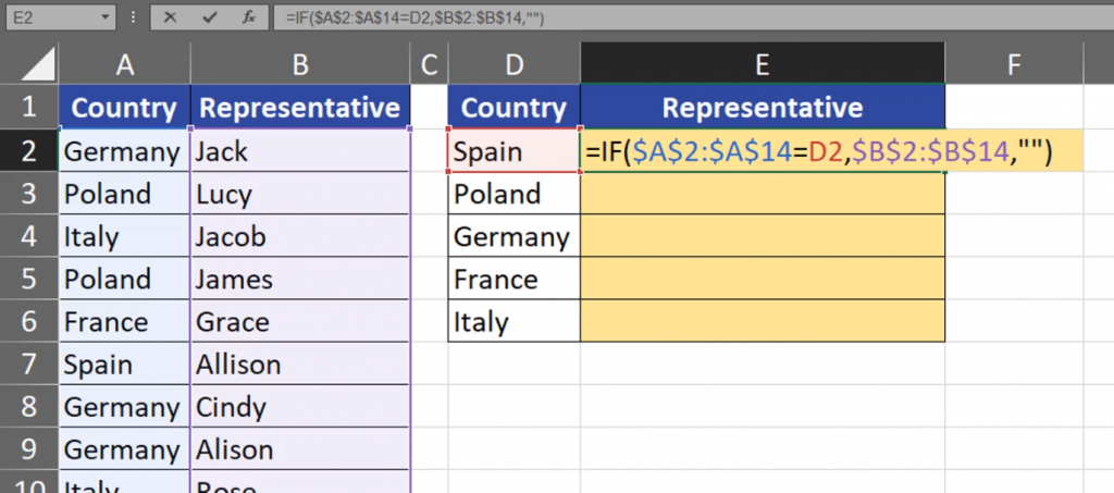
I will give you two solutions. The first solution will work from Excel 2019, and the second one will work in Dynamic Array Excel. First of all, we have to check if our representative comes from the country we are looking at. Let’s take a representative from Spain. There is only one representative of Spain in our example. We can check it using the IF function, where we have to create a proper logical test. We have to take into consideration the Country column, so let’s write it by selecting the column and clicking the F4 key to lock it. Then, we have to check if the values from the column are equal to just one country (Spain) by clicking the cell with the name of Spain (D4). It means that cell D4 will be compared to each cell from the Country column individually (Fig. 1)

The logical test will return TRUE only in the case of Spain. In the case of other countries, it will return FALSE. If the logical test is in an array, we can choose proper, corresponding result as a return value. We just need to select an array of the same size, which, in our case, is the Representative column. Then, we click the F4 key to lock it. When the logical test returns FALSE, we want to see an empty text string, so we have to write a space in double quotes. Let’s close the function with a parenthesis (Fig. 2)
=IF($A$2:$A$14=D2,$B$2:$B$14,” ”)
Since I’m working in Dynamic Array Excel, Excel spills the results to the whole column (Fig. 3).

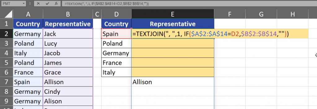
We can see that we have only one representative of Spain, and many empty cells. If we want to find the remaining representatives, we have to join the information we have. To do that, we can use the TEXTJOIN function, which is available from Excel 2019. We have to give the function a delimiter. Let’s write a comma and a space in double quotes. Then, we have to decide whether we want to ignore empty cells. We definitely do, so let’s write TRUE, or its shorter version, which is 1. Then, we just have to close the whole formula once again (Fig. 4).
=TEXTJOIN(“, “,1,IF($A$2:$A$14=D2,$B$2:$B$14,” ”))
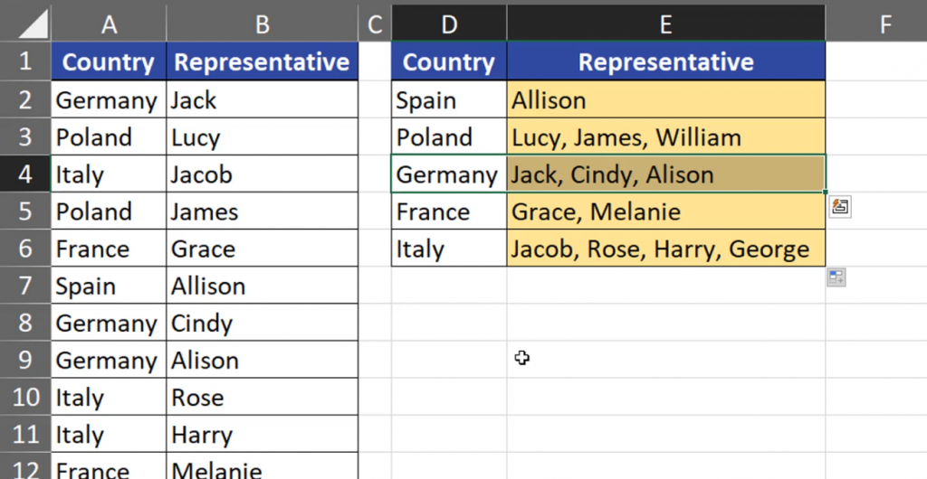
After entering the formula and copying it down, we have our results (Fig. 5).
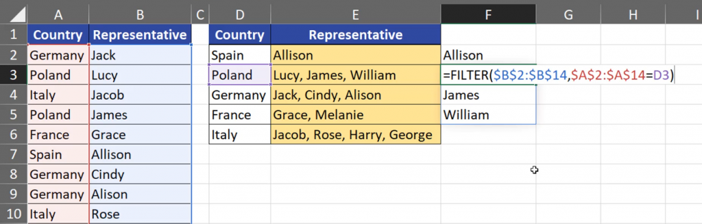
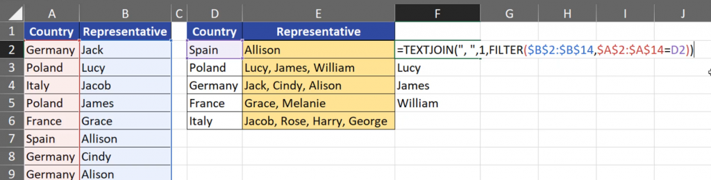
When we are in Dynamic Array Excel, we can use the FILTER function instead of the IF function. This function just filters our data. Let’s write FILTER function. Our data is located only in one column, which is the Representative column, so we have write the range and lock it with the F4 key. Then, we have to create an array of the same size with logical values of TRUE or FALSE. It means that we have to create the same logical test as we did with the IF function. Let’s add the Country column (A2:A14), F4 key to lock it, then an equal sign to check whether any of the value from the Country column is equal to Spain (D2). After closing it, we have a ready formula (Fig. 6).
=FILTER($B$2:$B$14,A$2:$A$14,=D2)

We can see that Spain has only one representative, but Poland has got three (Fig. 7).
That’s why we have to put our FILTER function results into the TEXTJOIN function. And, once again, we have to write a comma and a space in double quotes. Then, we have to decide that we want to ignore empty cells and close the whole formula (Fig. 8)
=TEXTJOIN(“, “,1,FILTER($B$2:$B$14,A$2:$A$14=D2))
We can see that the results in the first solution and in the second solution are the same (Fig. 9)
