Today, we are going to talk about the COUNTA function. This function counts almost everything, It counts formula results (Fig. 1),
COUNTA Function counting almost everythingFig. 1 Formula results
numbers written as text (Fig. 2),
Fig. 2 Numbers written as text
dates and time (Fig. 3),
Fig. 3 Dates and time
logical values (Fig. 4),
Fig. 4 Logical values
numbers (Fig. 5),
Fig. 5 Numbers
and errors (Fig. 6).
Fig. 6 Errors
It even counts a single number or value that we put as an argument to COUNTA function (Fig. 7)
Fig. 7 A number put as an argument
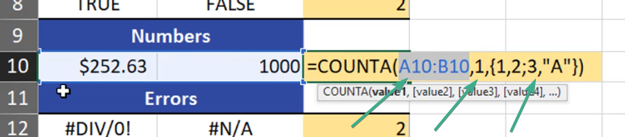
Let’s write an array with four elements. It doesn’t matter how many columns of rows this array has, but it’s important how many elements there are. So, we have a range of two cells with numbers, a single value and four elements (Fig. 8).
Fig. 8 A range, a single value and four elements
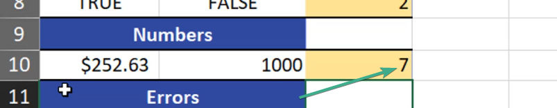
Since COUNTA function counts every element, it returns 7 (Fig. 9)
Fig. 9 The function returned 7
However, there is one thing that the COUNTA function doesn’t count. It doesn’t cells that are really empty. Cell A14 is really empty, however cell B14 isn’t. It has got a formula that returns an empty text string. COUNTA function counts an empty text string (Fig. 10).
Fig. 10 Empty text string
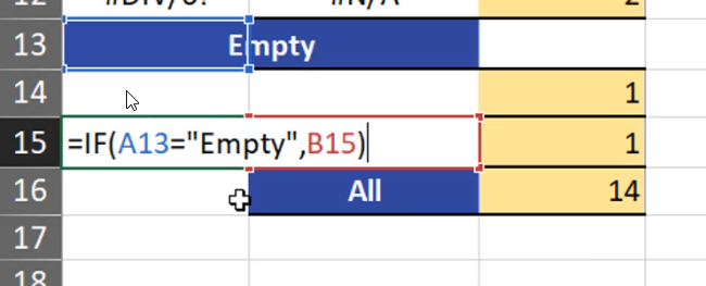
Even if a formula returns a value from an empty cell (B15), the COUNTA function will count cell A15 because it has got a formula (Fig. 11)
Fig. 11 A cell with a formula
The formula in cell B14 was counted by the COUNTA function (Fig. 12)
Fig. 12 A cell with a formula
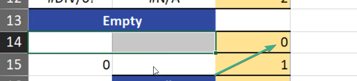
However, if we delete the formula, the COUNTA function will return 0 because cells A14 and B14 are now really empty (Fig. 13)
Fig. 13 Empty cells
Summing up, the COUNTA functions counts everything except for empty cells.
Sometimes, when we have formula results, we want to have only the text, i.e. the answer (Fig. 1).
Paste as values, the Paste Special windowFig. 1 — TRIM function results
We can copy the results, then right click a target cell and choose the Paste Values option from the pop-up menu (Fig. 2).
Fig. 2 — Pop-up menu — Paste values
And, we have just text not formula (Fig. 3).
Fig. 3 — Pasted values (text)
There is one more solution. When we copy our formula, we click on a target cell and press Alt + Ctrl + V combination to show the Paste Special window (Fig. 4). In the Paste area, we click Values, in the Operation area, we choose None, then we press OK.
Fig. 4 — Paste Special window
Now, we have the results only once. We don’t need the extra column, so we must delete it (Fig. 5)
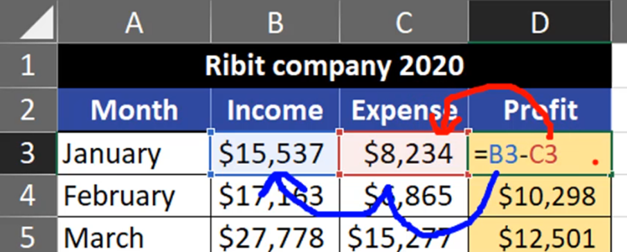
Today, we will discuss relative and absolute references. Let’s start with relative references to count a profit. If you want to count the profit, you just deduct expenses from income (Fig. 1).
Relative and absolute cell referencesFig. 1 — Source data
It means that you subtract the cell C3 value from the value in cell B3 (Fig. 2): =B3 — C3
Fig. 2 — Income minus expenses
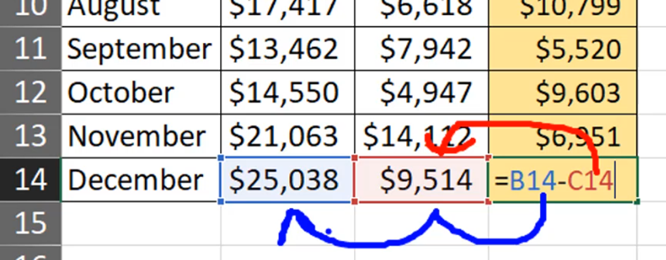
When we copy this formula down, it’s changing because we have different results in different cells. When we look at our formula, it refers to cells B3 and C3. But, in reality, it refers the cells which are one place to the left and two places to the left (Fig. 1). In the last formula (=B14-C14), we can see B14 minus C14 (Fig. 3) but it’s still one cell to the left and two cells to the left. The relative reference is moving with the formula and cell.
Fig. 3 — Formula change after copying down
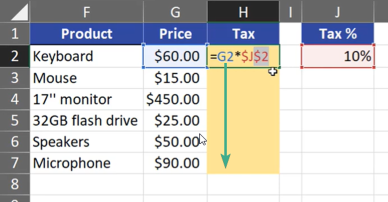
We don’t always want the formula to behave this way. In our second example you can see an absolute reference. We want to count the tax for each product. That’s why we have to multiply the price by our tax. However, we don’t want the tax cell to move, so we must lock cell J2 by pressing F4 key — add two $ signs (Fig. 4):
=G2*$J$2
Fig. 4 Tax calculations
When we copied our formula down, only cell G2 had changed because it’s a relative references. Cell J2 stayed the same and it will not move from this cell (Fig. 5)
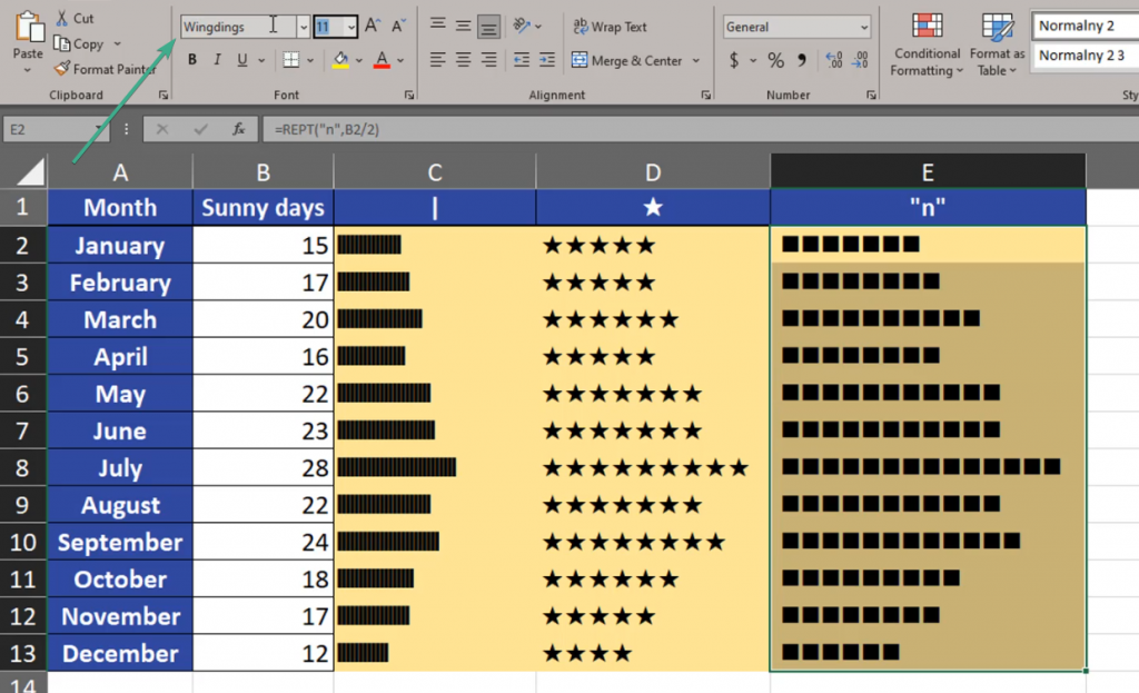
Today, we are going to talk about creating charts like data bars in cells using formulas. We want to create something like this (Fig. 1)
Data bars in a cell using character repeatFig. 1 Charts from data bars
Let’s start with creating a proper formula. We have to use the REPT (repeat) function. It will repeat a text, one or more chars, as many times as we write in the second argument. Let’s start with a pipe (a vertical line). We want to repeat it as many times as there are sunny days in a given month. Our formula looks like this (Fig. 2).
=REPT(“|”,B2)
Fig. 2 REPT formula with a pipe
After entering and copying down, we have data bars. However, the distance between individual signs is too big (Fig. 3)
Fig. 3 Data bars with too long distances
We have to narrow it by using, e.g. a different font that works with this sign. We are selecting our data bars and changing the font name to Script (Fig. 4). Now, it looks much better.
Fig. 4 Font change
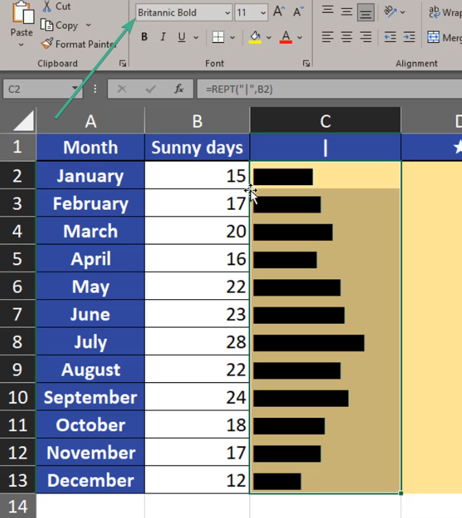
Let’s try, however, a different font. With Britannica Bolt, the signs look like real data bars (Fig. 5).
Fig. 5 Font change again
Let’s take the last example, which is the Haettenschweiler font. In my opinion, it looks the best, so I’m staying with this one (Fig. 6)
Fig. 6 The best font
Apart from repeating a pipe, we can repeat other signs. If they are wider than the pipe and if the number of repeats is too big, we may have a problem (Fig. 7)
=REPT(“*”,B2)
Fig. 7 A formula with an asterisk
We can see, that the asterisk string is too long (Fig. 8)
Fig. 8 Too long
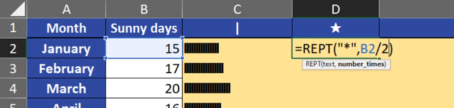
The solution is dividing the number, and the REPT function will only look at the integer part of the number. Let’s divide our numbers safely by two (Fig. 9).
=REPT(“*”,B2/2)
Fig. 9 Number division
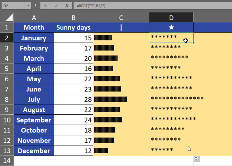
When there is a smaller number of repeats, it looks quite good (Fig. 10)
Fig. 10 Shorter strings
We have to remember that an asterisk is a simple sign, and we can use whatever sign we like. Let’s take, for example, a star (Fig. 11)
=REPT(“★”,B2/2)
Fig. 11 A formula with a star
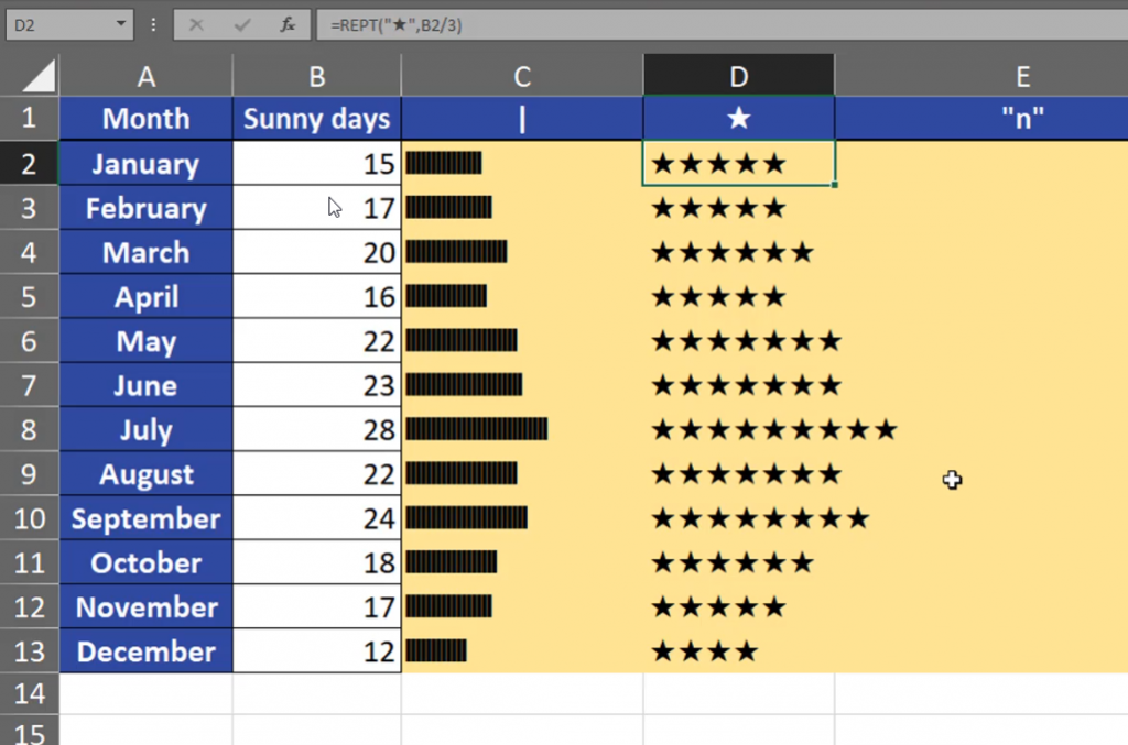
We can see that the strings are very long (Fig. 12). We can divide them by even a greater number, e.g. 3.
=REPT(“★”,B2/3)
Fig. 12 Dividing by 3
After putting the formula, it looks good (Fig. 13).
Fig. 13 Shorter strings
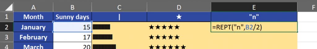
In our last example, we are going to repeat the letter n (Fig. 14)
=REPT(“n”,B2/3)
Fig. 14 Repeating n
Now, we can see many ns (Fig. 15)
Fig. 15 N string
However, we can change our font into Windings, and the letter n changes into squares, which looks quite good as data bars (Fig. 16)
Fig. 16 N into squares
Summing, up, when we use different signs and different number of repeats, we can create quite good data bars using a formula.
Today, we are going to talk about how to filter many pivot tables at once. We have three pivot tables based on the same dataset from the left (Fig. 1).
Filtering multiple Pivot Tables at once using a slicerFig. 1 Three Pivot tables
If we want to filter many pivot tables at once, we have to connect then into one slice. We have to select one cell from the first pivot table, then find the PivotTable Analyze tab and Insert Slicer command, where we want to add the slicer by Country (Fig. 2)
Fig. 2 Slicer by country
After pressing OK, we have the slicer. We can change its size and color (Fig. 3).
Fig. 3 Color and size change
Now, we can filter the first pivot table with the slicer. When we click on the name of a country, we can see changes in the first pivot table (Fig. 4). However, the second and the third pivot table did not change because they are not connected to the slicer.
Fig. 4 Slicer for the first pivot table
In order to connect then, we select the slicer, then we click on the Slicer tab, then the Report Connection command, which opens up a window, where we can see three pivot tables. They have generic, default names, and when we aren’t sure if they are the right ones, we can look which sheet they are located in. Then, we check proper check boxes to connect all pivot tables and press OK (Fig. 5)
Fig. 5 Connecting three pivot tables
Now, we can see that the slicer is filtering all, three, connected pivot tables (Fig. 6)
Fig. 6 Slicer for three pivot tables
When the pivot table name or the sheet name is not enough to identify the right one, we can change their names. When you select a proper pivot table, go to the PivotTable Analyze tab, then select the PivotTable Name command, and write the name you want. Let’s write PivotDate (Fig. 7). Giving names to pivot table makes it easier to work with them.
Fig. 7 Name change
Now, that we have the slicer, we can easily filter three pivot tables at once (Fig. 8).
Today, we are going to remove unnecessary spaces. Sometimes, there’s a space at the beginning of text, sometimes, there are more than one space between two words, and sometimes, there are some spaces at the end. The last ones are the hardest to notice (Fig. 1)
Remove unnecessary spaces — TRIM functionFig. 1 Unnecessary spaces
The name in the first line, Brave Brandon with a space at the end, is something different for Excel, than Brave Brandon without a space. In such a case, we want to use the TRIM function to remove the space (Fig. 2)
Fig. 2 TRIM function
After copying it down, we have our names without unnecessary spaces (Fig. 3)
Fig. 3 No unnecessary spaces
This simple function removes unnecessary spaces from the beginning, the end, and the middle of text beetween words only leaves one space.
Today, we are going to talk about extracting first names, middle names and last names from full names. We define the first name as the first word from the left, the last name as the first word from the right, and the middle name, as everything between those two. Middle names are a bit complicated, as they can may consist of one word, a space, an abbreviation, or two or more words (Fig. 1)
Extract First Last and Middle Name with FormulasFig. 1 A list of names
Let’s start with extracting the first name. We just have to use the LEFT function, which extracts signs from the left. We have to insert the FIND function there, so that it finds the first space, and write the space in double quotes (Fig. 2)
=LEFT(A2,FIND(“ “,A2))
Fig. 2 Extracting the first name
Now, we have the first name (Fig. 3).
Fig. 3 The first name
But, we have to remember that the FIND function will return the position of the sign we’re looking for, which means that it finds the 7th position, which is a space (Fig. 4).
Fig. 4 7th position
The first name , however, consists of only 6 letters, which is what we want. It means that we want to extract less letters. So, we have write the formula once again, but this time we subtract one sign (Fig. 5)
=LEFT(A2,FIND(“ “,A2)-1)
Fig. 5 Subtracting one sign
Now, we have only the first name without unnecessary signs. After dragging it down, the whole column is full (Fig. 6)
Fig. 6 Full column
Let’s go to last names. This case is a bit more complicated. We don’t know whether we’re looking for the first, the second, the third or even a more distant space (Fig. 7)
Fig. 7 Too many possible spaces
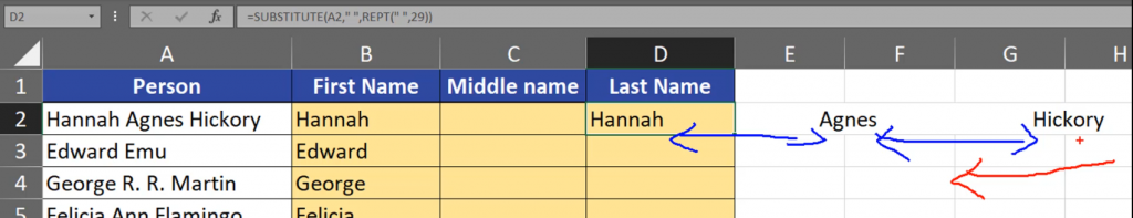
There’s a trick to solve it. We have to repeat spaces. Within our text, we have to substitute a single space into many spaces, let’s say 29. We use the REPT function (Fig. 8)
=SUBSTITUTE(A2,” “,REPT(“ “,29))
Fig. 8 Repeating spaces
After accepting our function, we have our changed names with many spaces between them (Fig. 9)
Fig. 9 Names with many spaces
Now, we can start extracting names from the right side. We’re extracting not only all signs from our name, but also the remaining 29 signs (Fig. 10).
=RIGHT(SUBSTITUTE(A2,” “,REPT(“ “,29)),29)
Fig. 10 Extracting name and 29 signs
Now, we have the last name and many, many spaces before it (Fig. 11)
Fig. 11 Name with spaces
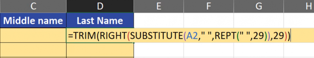
We have to delete them using the TRIM function. The TRIM function removes all spaces from a text string except for a single space between words. So, each space at the beginning and at the end of the string will be removed (Fig. 12)
=TRIM(RIGHT(SUBSTITUTE(A2,” “,REPT(“ “,29)),29))
Fig. 12 Trimming unnecessary spaces
After accepting it and copying it down, we have our last names (Fig. 13).
Fig. 13 Last names
Now, we have to find the thing between the first and the last name. We will use the SUBSTITUTE function. In the place of the first name, we will place nothing, i.e. an empty text string (Fig. 14).
=SUBSTITUTE(A2,B2,“”)
Fig. 14 Finding the middle name
Now, we have a shorter version of our name (Fig. 15).
Fig. 15 Shorter version
Let’s remove the last name now. We want to substitute the last name with an empty text string (Fig. 16)
=SUBSTITUTE(SUBSTITUTE(A2,B2,“”),D2,“”)
Fig. 16 Removing the last name
After entering and copying down, we have everything between the first name and the last name (Fig. 17). As you can see, we have also extracted spaces which we don’t need. So, let’s use the TRIM function to delete unnecessary spaces.
=TRIM(SUBSTITUTE(SUBSTITUTE(A2,B2,“”),D2,“”))
Fig. 17 Unneeded spaces
Because we are editing whole column we can press Ctrl + Enter.
That’s how we extract first names, last names and everything in between with appropriate formulas.
Today, we are going to extract middle names from full names. However, not everybody has got a middle name, so let’s start with the first and the last name. We can use here the Flash Fill option, which means that we just have to start writing the first name, then another first name. After that, the Flash Fill command does the work for us (Fig. 1).
Extract middle names with Flash FillFig. 1 — Using the Flash Fill option
All we need to do is accept the results with Enter, and we have the first names (Fig. 2)
Fig. 2 — Entering the results
We do the same with the last name, i.e., we start writing the last name in the first cell, but this time we will force the Flash Fill option to work by pressing the Ctrl + E keyboard shortcut (Fig. 3). This way, we have last names (Fig. 4)
Fig. 3 — Flash FillFig. 4 — Flash Fill results
Now, the hardest part – middle names. We start writing the middle name in the first row, however, we don’t have a middle name in the second row. This time we’ll also use the Flash Fill option (Fig. 5)
Fig. 5 — Flash Fill for middle names
When all middle names have been extracted, we can see an error. Edward isn’t a middle name. We have to correct the Flash Fill answer. We can do it, until the Flash Fill Options icon is showing up (Fig. 6).
Fig. 6 — Flash Fill icon
We have to change the middle name, which, in fact, isn’t a middle name, for a different mark, e.g. an exclamation mark. We simply write the mark in the place of the error, press Enter, and the Flash Fill option will do its magic again (Fig. 7) Exclamation marks are in the rows, where there aren’t middle names.
Fig. 7 — Exclamation marks
We can put almost anything in the place of the exclamation mark, e.g. a star (Fig. 8).
Fig. 8 — Stars
We usually don’t want any stars or other signs. We want to have blank cells, however, the Flash Fill option doesn’t work with spaces. That’s why we can use the Filter option, which we can find in the Data tab (Fig. 9). In the Filter option, we want to show only this sign (a star).
Fig. 9 — Filter option
Now, we’re left only with stars (Fig. 10). We have to select the range (Ctrl + Shift + ↓) and press the Delete key to delete all the signs.
Fig. 10 — Selected range
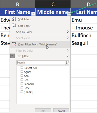
Then we can turn off the filter. We can do it manually, by pressing the filter icon and selecting the Clear Filter From “Middle names” option (Fig. 11) or by pressing the Ctrl + Shift + L key combination.
Fig. 11 — Turning off the filter
Now, we have middle names only in places, where they really exist, and blank cells, where there aren’t any middle names (Fig. 12)
Today, we will discuss logical tests and the IF function in Excel.
IF function and logical tests
Let’s start with logical test. We want to check whether our students passed the test, i.e. whether they achieved 70 points (cell D2). We need a formula that checks if the number from cell B5 is greater or equal to the value from in cell D2. We aslo have to lock the value from cell D2 by pressing F4 key (Fig. 1).
Fig. 1 — Logical test with locked cell D2
After copying the formula down, we have our logical answers (Fig. 2)
Fig. 2 — Logical answers
Logical answers, however, aren’t human answers. If we want something simpler, like pass/fail, we need to use the IF function in cell D5 (Fig. 3).
Fig. 3 — IF function inserting simpler answers
After copying it down, we have the answers that we want, instead of logical ones. If the logical test returns False, our IF function returns text Fail. If the logical test returns True, our IF function returns text Pass (Fig. 4)
Fig. 4 — Simpler/human answers
Sometimes, we want to know how many more points a student needs to pass their exam. In that case, we also use the IF function. This time, however, we are changing the direction of our test. We need to check if the value from cell B5 is lower than the value from cell D2 (70 points). If it is lower, it means that the student failed the exam. Calculating the number of missing points is a simple, mathematical operation. We just have to subtract the value from cell B5 (62 points) from the value in cell D2 (70 points). However, if a student passed the exam, we don’t need to calculate anything, so we’re returning 0 points (Fig. 5).
=IF(B5<$D$2,$D$2‑B5,0)
Fig. 5 — IF function calculating the number of missing points
After copying it down, we can see that one student needs 8 points to pass, and another one needs 35. The students who passed the exam, don’t need any more points, that’s why IF function returned 0 for them (Fig. 6).