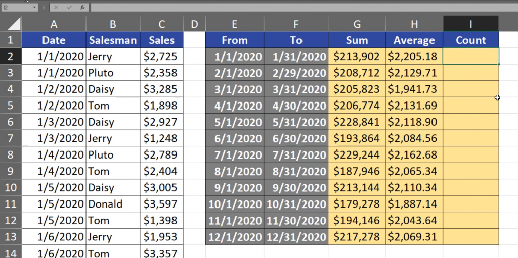
Today, we are counting sums, averages and number of transactions with more than one condition. In our example, we have transaction sales table and we want to count the values for given months. However, the months are written as the first day of the month and the last day of the month. It means that we have to add two conditions in order to count it. Let’s start with sums. We can use the SUMIFS function. The first argument of this function is a range on which we will be summing. In our case it’s the sales column so we have to select cell C2 and press the Ctrl + Shift + ↓ combination, then the F4 key to lock it (Fig. 1).
=SUMIFS($C$2:$C$1193
SUMIFS AVERAGEIFS and COUNTIFS functions SUM with conditionsFig. 1 SUMIFS function with a locked range
We write a comma, and then we are going to the criteria range 1. This will be the range where we will be checking the first criterion, which is the third argument of the SUMIFS function. In our case, we are checking dates, so let’s press cell A2, Ctrl + Shift + ↓, then the F4 key. We are adding a comma again, and now we have to write the first condition, which is the first criterion. The order of our conditions is not important because, in the end, all conditions have to be met to count the thing we want. Let’s start with the From date. We want values that are bigger or equal to this date, which means that we have to write the symbols of larger than and equal in double quotes, then an ampersand because we are combining this text with the value from cell E2 (Fig. 2).
=SUMIFS($C$2:$C$1193,$A$2:$A$1193,”>=”&E2
Fig. 2 SUMIFS with the first condition
After pressing the F9 key, we can see that Excel changed the date into a number. This makes Excel check our condition properly (Fig. 3).
=SUMIFS($C$2:$C$1193,$A$2:$A$1193,“>=43831”
Fig. 3 Excel changed the dates
However, let’s move back to previous text by pressing Ctrl + Z. Now, we have the first condition. We can see that the second condition is necessary with second critirion because the next two arguments are in square brackets (Fig. 4).
=SUMIFS($C$2:$C$1193,$A$2:$A$1193,”>=”&E2
Fig. 4 Arguments in square brackets
Criteria range 2 in our case is the same as criteria range 1, so we can just copy it (Ctrl +C, Ctrl +V), but we really need to put it because each criteria range is working just with the argument of its criteria. It means that criteria range 1 is working with criteria 1, and criteria range 2 is working with criteria 2. In our case, the criteria 2 are numbers smaller than or equal to the last day of the month in cell F2.
When we want to sum the values from the sum range, the first and the second condition have to be met. Let’s put the formula and copy it down. We can see that at the end everything is working properly because we have written the formula properly (Fig. 6).
Fig. 6 Proper results
We still have some more values to count. Let’s take the averages. Since I’m a lazy person, I will copy the whole formula in edit mode, then go to the Average column, paste it and change only the name of SUMIFS into AVERAGEIFS. After entering it, we can see that only the sum range changed its name into average range. The remaining argument names stayed the same. It’s because the SUMIFS and the AVERAGEIFS formulas have the same syntax, but they count sums and averages correspondingly (Fig. 7).
Fig. 7 Function name change
Let’s put the formula into our cell and copy it down. We have the results (Fig 8).
Fig. 8 SUMIFS reults
Let’s now count the number of transactions. We will use the COUNTIFS function. This function doesn’t have any range on which we could count sums, averages and so on. It only needs criteria ranges and criteria. Our first criteria was the one with dates. So, let’s write A2, then press Ctrl + Shift + ↓, then the F4 key to lock it and a comma. I want to show you that the order of conditions is not important. Let’s take values smaller that or equal to the date in cell F2, comma, then the same criteria range, then the second criteria will be greater than or equal to the value from cell E2. Those are all the arguments we need for a COUNTIFS function (Fig. 9).
After copying the formula down, we have the results. We can check if our average is correct just by looking at it because it is just the sum divided by the number of transactions (Fig. 10).
Fig. 10 Checking the results
We can see that the numbers are exactly the same as in the Average column (Fig. 11).
Fig. 11 AVERAGEIFS and divide gives the same results
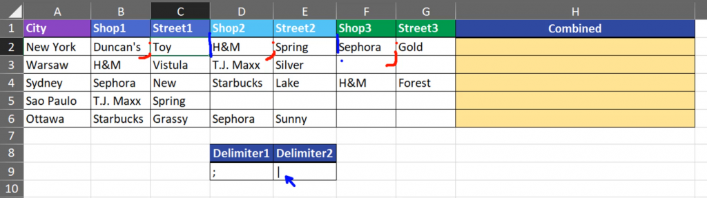
Today, we are going to combine text with two, different delimiters. In our example, we have shop and street names. We want to put a semicolon between each shop and street name. However, between street and shop names we want to put another symbol, which is a pipe. What is important in our example, is the fact that not all cells are filled. We want to just ignore them while combining text (Fig. 1).
Combine text with different delimitersFig. 1 — Text to combine
This task is very simple in Excel 2019 and newer versions because we have the TEXTJOIN function. In the first argument of this function, we are putting the delimiter. We can even put more than one delimiter. In our example, the delimiters are placed in cells D9 and E9, so let’s put them in the formula and let’s lock them by pressing the F4 key. When we put more than one delimiter in the TEXTJOIN function, the function will use them alternatively, which means that first, it will use the semicolon, then the pipe, then the semicolon and so on. In next argument we have to decide whether we want to ignore empty cells or not. In this case, as I said earlier, it’s very important for us to ignore them, so we are writing TRUE or 1. The last argument we need is just text, i.e. the range with text. Let’s close the formula (Fig. 2)
=TEXTJOIN($D$9:$E$9,1,B2:G2)
Fig. 2 — Formula for combining text
After putting it into the cell, let’s copy it down. We have the results. We can see there are semicolons between shop and street names, and pipes between street and shop names (Fig. 3).
Fig. 3 — Combined text
In the TEXTJOIN formula, delimiters orientation is not important. They can be horizontal or vertical.
We can even hardcode them here by selecting first argument and pressing the F9 key to evaluate it. Now, they are written as text (Fig. 4).
=TEXTJOIN({“;”,”|”},1,B2:G2)
Fig. 4 — Hardcode delimiters
We can leave them like that and the formula will work the same.
Today, we are going to combine or concatenate two or more texts together. Let’s start with creating full names. It is a simple example with two texts. We can use the CONCATENATE function, or, if you have Excel 2019 or a newer one, you can just use the CONCAT function which combines two text ranges. The CONCATENATE function cannot combine ranges, only single cells. However, in our example, it doesn’t matter because when we combine the first name and the last name, in reality, we want to combine three texts as there is a delimiter between the first and last name. That’s why we have to add, let’s say, a space. The space should be in double quotes because it is a text (Fig. 1).
Combine Text from Two or more Cells
=CONCATENATE(A2,” “,B2)
Fig. 1 CONCATENATE function
After entering and copying it down, we have full names (Fig. 2).
Fig. 2 Full names
If you don’t like using the function, you can use the ampersand sign (&) to combine texts. However, while using the sign, it is important to put the sign between each point of connection. It means that the & sign must be placed between the first cell address and the space, and between the space and another cell address (Fig. 3)
=A2&” “&B2
Fig. 3 Ampersand signs in a formula
After entering the formula, we have the same results as after using a function (Fig. 4). It is up to you which one you choose.
Fig. 4 The same results
In our second example, we want to combine more than one text together, i.e., the first, middle and last name. We will use the CONCATENATE function once more, but this time we are clicking on the insert function command near the formula bar and we can see that a Function Argument window appeared. In the window, we have argument/text boxes where we will write our text. We can choose a text from a cell (press Tab). In the Text2 bar, we can write a space. When we press the Tab key, Excel will add double quotes for us. In the Text3 bar there will be cell B2. In the next bar below, we do the same with writing a space. In the last bar, we place cell C2. We can even see our formula result straight in the Function Window (Fig. 5).
=CONCATENATE(A2,” “,B2,” “,C2)
Fig. 5 Function Arguments window
After entering the formula, we have our results (Fig. 6). In this example, using the Insert Function command was quite fast.
Fig. 6 Formula results
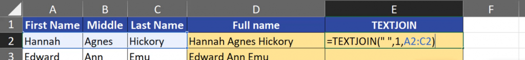
I have also prepared one more function that exists from Excel 2019. It is called TEXTJOIN. It can combine text from ranges with the same delimiter. In our case, the delimiter is a space, so we have to write a space in double quotes. Then, we have to decide if we want to ignore empty cells. In most cases yes, so we can write either TRUE or 1. Let’s write 1 because it is shorter. Then, we are selecting the text range, which is the cells that we want to join (Fig. 7)
=TEXTJOIN(“ “,1,A2:C2)
Fig. 7 TEXTJOIN function
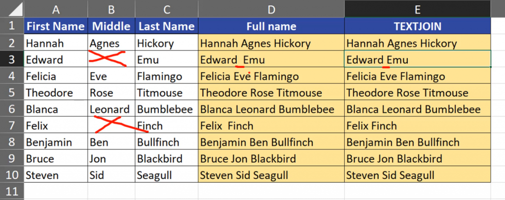
After entering the formula and copying it down, we have our results (Fig. 8)
Fig. 8 TEXTJOIN function results
While combining many texts, it is very important to choose proper function. Let’s assume that some people don’t have middle names. In such a case, the TEXTJOIN function will ignore empty cells and will add only one space. However, the CONCATENATE function will leave two spaces. In such a situation we would have to use the IF function to properly address this problem (Fig. 9).
Fig. 9 One space and two spaces in different functions
Summing up, we joined the first, middle and last name in each row using the CONCATENATE function that combines more than two texts, and the TEXTJOIN function that combines a range of texts.
When you want to count the number of columns in a range, you can use the COLUMNS function and select a proper range (Fig. 1)
COLUMNS function — how many columns in a range
=COLUMNS(B13:E17)
Fig. 1 COLUMNS function
The function will return the number of columns in this range (Fig. 2)
Fig. 2 Number of columns
You can also create a horizontal sequence of numbers. You just have to write the COLUMNS function and create a proper range, let’s say B13 to B13. In this case, it is important to lock one of the cells with a $ sign by pressing the F4 key so that it doesn’t move (Fig. 3)
=COLUMNS($B$13:B13)
Fig. 3 COLUMNS function with a range
After entering the formula and copying to the right, we can see that our range expands, i.e. one cell stays the same, and the other one is moving to the right (Fig. 4).
Today, we are going to count sums and averages with conditions. In our first example, we have a small table where we sell fruit. We want to sum up the whole weight and average weight for a single cell. To sum the values with conditions we can use the SUMIF function. In the first argument, we write the range where we need to check our condition and lock it by pressing the F4 key. In the second argument, which is criteria, we just put a reference to a single cell with the product name. We don’t have to lock the cell because while copying the formula down, we want the fruit names to change. The third argument of the function is the sum range. It is closed in square brackets which means that it is not necessary write it, however we will do it. We want to sum values from the Weight column. Then the F4 key to lock it (Fig. 1).
SUM and AVERAGE with condition — SUMIF and AVERAGEIF functions
=SUMIF($B$2:$B$10,F2,$C$2:$C$10)
Fig. 1 SUMIF function
After all arguments have been written, let’s look at our ranges and try to understand how the SUMIF function works. The function will look at each cell in the Product column and check if they meet the conditions. In the first cell, we have apples, which means that the condition is met. In such a situation, the function will keep on looking for the third argument placed in the same row. If it finds it, it will add the value. If there is another cell that meets the same condition, it will also add the value from the same row (Fig. 2).
Fig. 2 Finding conditions
Our formula looks as follows (Fig. 3).
=SUMIF($B$2:$B$10,F2,$C$2:$C$10)
Fig. 3 SUMIF formula
After entering and copying down, we can see how many apples, pears and oranges we have sold (Fig. 4).
Fig. 4 Results
Now, let’s try to count the average weight of a single sale. We just have to copy our SUMIF formula in the edit mode and paste it into the cell in the Average column. The SUMIF and the AVERAGE functions have the same arguments. We just change the function name. We can see that the name of the third argument changed from sum range into average range, however it is still the same Weight column (fig. 5).
=AVERAGEIF($B$2:$B$10, F2,$C$2:$C$10)
Fig. 5 Name change
After entering and copying it down, we have our results (Fig. 6).
Fig. 6 AVERAGEIF counted
Let’s move on to our second example. We want to check here what would happen if we give the AVERAGEIF or SUMIF function just two arguments. In this example, we just want to count the average sale. We are starting with a simple AVERAGE function without conditions, so without IFs, for the Sales column (Fig.7).
=AVERAGE(C2:C11)
Fig. 7 Simple AVERAGE function
After entering it, we have the average (Fig. 8).
Fig. 8 Average
Now, let’s count the average with a condition. We don’t want to count the value if it equals 0. Let’s write the AVERAGEIF function, select the same range and write the condition. We open double quotes and write <>0 and close it. When we don’t write the third argument in the AVERAGEIF or SUMIF functions, Excel takes the first range as the range in which we are doing our calculations. In this situation Excel doesn’t take empty cells and cells with 0 into calculating the average. After entering it, we can see different results. It’s because our condition was triggered in the AVERAGEIF function, which means that Excel did not count the cells with 0 (Fig. 9).
Fig. 9 Different results
When we delete the value with 0, we can see that the AVERAGE and AVERAGEIF function return the same results. It’s because functions such as AVERAGE, SUMS, MIN and MAX do not consider empty cells (Fig. 10).
Fig. 10 Results without empty cells
However, when we put 0 into the cells, the AVERAGE function will count it which means that the average will go down (Fig. 11).
Fig. 11 Results with zeros
Summing up, a simple AVERAGE function counts cells with 0, and the AVERAGEIF function doesn’t due to the condition.
In Excel, in most situations, empty cells are treated as 0.
Today, we want to count how many times we sold apples, pears and oranges. We are going to use a small table to check our results, because with a bigger table it isn’t going to be easy. We will use the COUNTIF function. This function has got only two arguments. The first one is a range, where we will be checking our conditions or criteria. In our case, the criterion is the name of our product, so we are selecting the cell with the product name. Such a function will check each cell in the range, whether it contains the name or not.
COUNTIF function — how many times we sell apples
=COUNTIF(B2:B10,F2)
Fig. 1 COUNTIF function
If a cell contains the name, the function will add 1 to the counter. We can see that there are four 1s.
Fig. 2 Four 1s
We also have to lock the range by pressing the F4 key, so that it stays in the same place. Criteria, however, should not be locked because we want them to change while copying the formula down, i.e. we want a given product to change.
=COUNTIF($B$2:$B$10,F2)
Fig. 3 Locked range
After entering and copying down, we have our results. We can see that apples have been sold four times, pears three times and oranges two times. It will also work with bigger tables. All we need to do is to write a bigger range.
Today, we are going to talk about choosing a random element from a list without repeats. We have eight elements in our list. I put there the same number two times, which gives me the opportunity to choose the same number two times. If there are three the same numbers, I could choose the number up to three times. However, the choosing is random, so I don’t really know how many times I will choose it.
Random list no repeats, manual and formulas solutionsFig. 1 A list of elements
If we want to choose an element from the list at random without repeats, we can use a manual solution. We need to write the RAND function which returns numbers from 0 to 1 with fifteen digit precision. It means that it’s almost impossible to choose the same number twice (Fig. 2).
=RAND()
Fig. 2 RAND function
After dragging formula down, we have 8 random numbers. We have to remember that the RAND function is a volatile function. It means that it is recalculated every time our worksheet changes (Fig. 3).
Fig. 3 Recalculation
Now, that we have our helper column, we can do the sorting. We go to Data tab and we choose the A to Z or Z to A command.
Fig. 4 Sorting
If we want to have, e.g. five elements, we have to choose five elements from the top. It doesn’t matter whether we sort from A to Z or Z to A. We just choose the first five elements. We can see that the numbers are recalculated every time we sort our data (Fig. 5)
Fig. 5 Five elements from the list
Let’s get back to our original list and try the second solution. It is from Legacy Excel and it uses formulas. Let’s start with a way to sort our numbers. We can use, e.g. the LARGE function, which returns the biggest number from the list, then the second biggest, then the third biggest, and so on. We have to press the F4 key to lock our list. Then, we need a way to choose the first, the second, and so on numbers. So, we want to change our key argument using a proper function. One of the simplest solution I know is using the ROW function with reference to cell A1, which is free (without $ signs). When we copy our formula down, our A1 reference will also go down, and the ROW function will return the first row, the second, the third, and so on (fig. 6)
=LARGE($B$2:$B$9,ROW(A1))
Fig. 6 ROW function
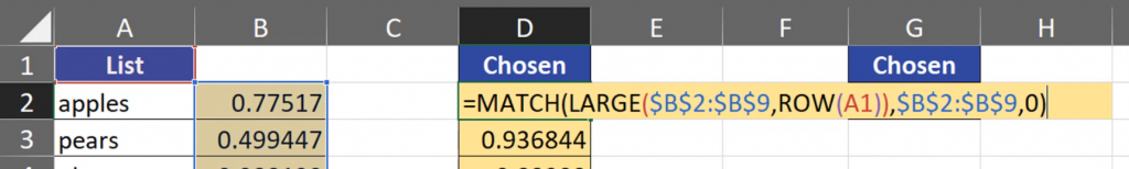
After entering the formula, we have our numbers placed from the largest to the smallest. Our five elements are now in a proper order. It means that now we can choose elements. However, we must use the MATCH and INDEX function in our data orientation. Let’s add the MATCH function to find the position of our number. We have to add the range, which is our random number column and press the F4 key to lock it. Then, we are adding 0 because we want to have the exact match (Fig. 7)
=MATCH(LARGE($B$2:$B$9,ROW(A1)),$B$2:$B$9,0)
Fig. 7 MATCH function
After entering and copying down, we have positions of the largest numbers. When we look at the first position in our Chosen column, we have 5. It means that the largest number from our original list is located in the 5th place.
Fig. 8 Position of the largest number
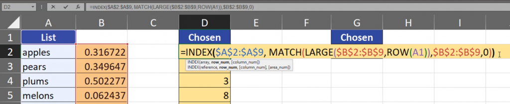
However, we don’t want to have position numbers, but the elements connected to those numbers. It means that we have to add the INDEX function to our MATCH function. This time, we want to choose elements from our list, so we are adding the range and lock it by pressing the F4 key. It turns out that our MATCH function is the row number. We have to close the formula (Fig. 9)
After entering and copying down, we have elements selected at random without repeats. When I press the F9 key, I am forcing it to recalculate our results. Sometimes, we see our number (123) twice because it is twice on our original list (Fig. 10)
Fig. 10 Elements selected at random
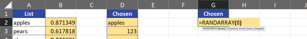
It’s high time we tried the final solution in Dynamic Array Excel. This solution is simpler that the one in Legacy Excel because we just need two functions. In DA Excel, we have the RANDARRAY function which can create a random array. We just need to copy the same column into our formula, which means that we need an array with eight rows and one column. That’s why we are writing just 8 (Fig. 11).
=RANDARRAY(8)
Fig. 11 RANDARRAY function
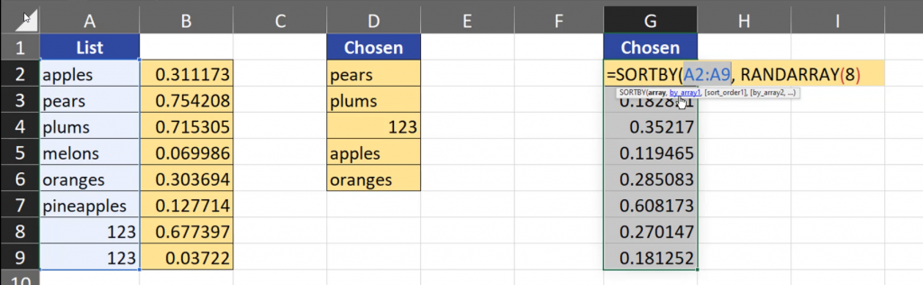
After putting our formula into Excel, we have eight random numbers. In DA Excel, we can sort by this column. Thus, we have to add the SORTBY function to our formula. The array which we want to sort is our list. This time, we don’t have to lock it because it is a DA formula, and our formula is the result (Fig. 12).
=SORTBY(A2:A9,RANDARRAY(8))
Fig. 12 SORTBY function
After putting the formula down, we have eight elements from our list in a random order. Pressing the F9 key allows us to choose elements once again at random. Let’s choose five elements from the top once again. We still can see the remaining elements. If you don’t want to see them, you have some options. You can, for example, select five elements from our list, then press the F2 key to go to the formula edit mode, then press the Ctrl + Shift + Enter combination to create an array formula. The array formula is from Legacy Excel. Now, we have only five elements because I’ve selected only five cells. Those cells are an array, which means that we cannot change or delete any single element of the array. If you want to change it, you have to change the whole array at one time (Fig. 13).
Fig. 13 An array
Summing up, if you want to choose an element at random from a list, you can use a manual solution, a Legacy Excel solution or a Dynamic Array solution.
When you want to count the numbers of rows in a range, you can use the ROWS function. This function looks only at rows in a given range, and in the end, it returns the numbers of rows from the selected range.
ROWS function, how many rows in a range
=ROWS(B11:C16)
Fig. 1 ROWS function for a given range
The ROWS function allows you also to create a sequence of numbers. We just have to select a proper range (from cell C11 to C11) (Fig. 2), but we have to lock the first C11 cell with a $ sign.
=ROWS($C$11:C11)
Fig. 2 Locking the cell
Then, we copy the formula down. We can see that our range keeps expanding because the first cell stayed the same, and the second cell keeps moving down (Fig. 3)
Today, we are going to talk about mixed cell references and we will start with the simplest example, which is the multiplication table. Multiplication is simple. We just have to multiply the row header by the column header. We are going to write a formula in cell B3, then we are going to copy the formula down and to the right. First, we are referring to cell A3. Then we have to ask ourselves how our reference should change while copying it down and to the right. Let’s look at our data which we will be referring to. We’re starting with row headers. Our row headers are in one column and many rows (Fig. 1).
It means that the rows are changing but the columns stay the same. Thus, we have to lock the column name, not the row number. We can use the F4 key which cycles through cell reference types. It turns out that we had to press the F4 key three times, so that the $ sign is before the column name, not before the row number (Fig. 2).
=$A3
Fig. 2 Locked column name
It means that the column name should stay the same, but the row number should change. We want to multiply them so we are adding cell B2. Let’s look at the headers once again. As we can see, our column headers are placed in one row, but many columns.
=$A3*B2
Fig. 3 Column headers on one row
This time, we want to lock the rows, not the columns. We have to click the F4 key two times, so that the $ sign is before the row number, not the column name, which means that the rows should stay the same, but the columns should change (Fig. 4).
=$A3*B$2
Fig. 4 Locked row number
After entering the formula, copy it down and to the right. We can see that the results are proper (Fig. 5)
Fig. 5 Proper results
Let’s check the last cell. We can see that we have proper cell reference to row headers, as we still refer to column A, and the rows changed. Analogically, for column headers, we can see that the columns changed, and the row stayed the same (Fig. 6).
Fig. 6 Proper cell reference
That’s how mixed cell reference works. It will work in many different examples, like the one below. We have to divide profits for shareholders. The situation is analogical. Our profits are in one column and many rows (Fig. 7)
Fig. 7 Profits in one column
We have to lock the column name, i.e. the $ sign should be placed before the column name, not before the row number. Then, we want to multiply it by percentages. They are in one row — row number 3, which shouldn’t change (Fig. 8).
=$B6*
Fig. 8 Percentage in one row
So, when we refer to cell C3, we have to lock the rows, not the columns because they are changing. Let’s press the F4 key twice and lock the rows (Fig. 9).
=$B6*C$3
Fig. 9 Cell C3 reference
After copying the formula down and to the right, we have proper results.
Today, we are going to talk about copying cell formatting from one cell to another. We just have to click a given cell, then go to Home tab, press the Format Painter command and click on the cell to which you want to copy the formatting (Fig. 1).
Format Painter — How to copy cell formattingFig. 1 Copying from one cell to another
The Format Painter can also copy the formatting from more than one cell. We just select the cells, then click on the Format Painter, then select the range to which you want to copy the formatting, and enter it (Fig. 2).
Fig. 2 Copying to more that one cell.
When you select a cell range and you double-click the Format Painter command, the copying process is going until you press the Esc key. You can even go to other sheets, and copy the formatting there.