Today, we want to count how many times we sold apples, pears and oranges. We are going to use a small table to check our results, because with a bigger table it isn’t going to be easy. We will use the COUNTIF function. This function has got only two arguments. The first one is a range, where we will be checking our conditions or criteria. In our case, the criterion is the name of our product, so we are selecting the cell with the product name. Such a function will check each cell in the range, whether it contains the name or not.
COUNTIF function — how many times we sell apples
=COUNTIF(B2:B10,F2)
Fig. 1 COUNTIF function
If a cell contains the name, the function will add 1 to the counter. We can see that there are four 1s.
Fig. 2 Four 1s
We also have to lock the range by pressing the F4 key, so that it stays in the same place. Criteria, however, should not be locked because we want them to change while copying the formula down, i.e. we want a given product to change.
=COUNTIF($B$2:$B$10,F2)
Fig. 3 Locked range
After entering and copying down, we have our results. We can see that apples have been sold four times, pears three times and oranges two times. It will also work with bigger tables. All we need to do is to write a bigger range.
Today, we are going to talk about choosing a random element from a list without repeats. We have eight elements in our list. I put there the same number two times, which gives me the opportunity to choose the same number two times. If there are three the same numbers, I could choose the number up to three times. However, the choosing is random, so I don’t really know how many times I will choose it.
Random list no repeats, manual and formulas solutionsFig. 1 A list of elements
If we want to choose an element from the list at random without repeats, we can use a manual solution. We need to write the RAND function which returns numbers from 0 to 1 with fifteen digit precision. It means that it’s almost impossible to choose the same number twice (Fig. 2).
=RAND()
Fig. 2 RAND function
After dragging formula down, we have 8 random numbers. We have to remember that the RAND function is a volatile function. It means that it is recalculated every time our worksheet changes (Fig. 3).
Fig. 3 Recalculation
Now, that we have our helper column, we can do the sorting. We go to Data tab and we choose the A to Z or Z to A command.
Fig. 4 Sorting
If we want to have, e.g. five elements, we have to choose five elements from the top. It doesn’t matter whether we sort from A to Z or Z to A. We just choose the first five elements. We can see that the numbers are recalculated every time we sort our data (Fig. 5)
Fig. 5 Five elements from the list
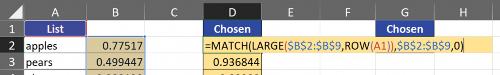
Let’s get back to our original list and try the second solution. It is from Legacy Excel and it uses formulas. Let’s start with a way to sort our numbers. We can use, e.g. the LARGE function, which returns the biggest number from the list, then the second biggest, then the third biggest, and so on. We have to press the F4 key to lock our list. Then, we need a way to choose the first, the second, and so on numbers. So, we want to change our key argument using a proper function. One of the simplest solution I know is using the ROW function with reference to cell A1, which is free (without $ signs). When we copy our formula down, our A1 reference will also go down, and the ROW function will return the first row, the second, the third, and so on (fig. 6)
=LARGE($B$2:$B$9,ROW(A1))
Fig. 6 ROW function
After entering the formula, we have our numbers placed from the largest to the smallest. Our five elements are now in a proper order. It means that now we can choose elements. However, we must use the MATCH and INDEX function in our data orientation. Let’s add the MATCH function to find the position of our number. We have to add the range, which is our random number column and press the F4 key to lock it. Then, we are adding 0 because we want to have the exact match (Fig. 7)
=MATCH(LARGE($B$2:$B$9,ROW(A1)),$B$2:$B$9,0)
Fig. 7 MATCH function
After entering and copying down, we have positions of the largest numbers. When we look at the first position in our Chosen column, we have 5. It means that the largest number from our original list is located in the 5th place.
Fig. 8 Position of the largest number
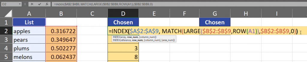
However, we don’t want to have position numbers, but the elements connected to those numbers. It means that we have to add the INDEX function to our MATCH function. This time, we want to choose elements from our list, so we are adding the range and lock it by pressing the F4 key. It turns out that our MATCH function is the row number. We have to close the formula (Fig. 9)
After entering and copying down, we have elements selected at random without repeats. When I press the F9 key, I am forcing it to recalculate our results. Sometimes, we see our number (123) twice because it is twice on our original list (Fig. 10)
Fig. 10 Elements selected at random
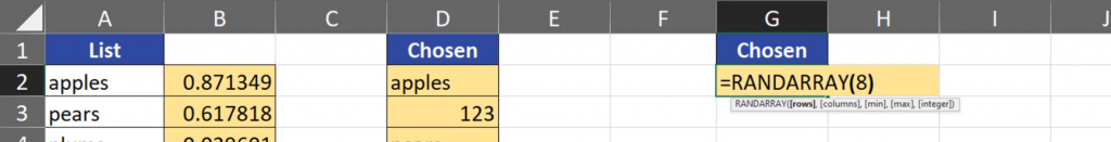
It’s high time we tried the final solution in Dynamic Array Excel. This solution is simpler that the one in Legacy Excel because we just need two functions. In DA Excel, we have the RANDARRAY function which can create a random array. We just need to copy the same column into our formula, which means that we need an array with eight rows and one column. That’s why we are writing just 8 (Fig. 11).
=RANDARRAY(8)
Fig. 11 RANDARRAY function
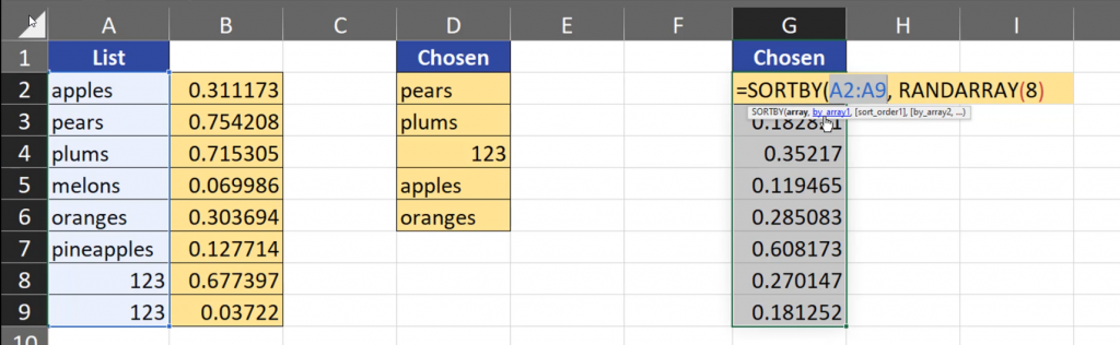
After putting our formula into Excel, we have eight random numbers. In DA Excel, we can sort by this column. Thus, we have to add the SORTBY function to our formula. The array which we want to sort is our list. This time, we don’t have to lock it because it is a DA formula, and our formula is the result (Fig. 12).
=SORTBY(A2:A9,RANDARRAY(8))
Fig. 12 SORTBY function
After putting the formula down, we have eight elements from our list in a random order. Pressing the F9 key allows us to choose elements once again at random. Let’s choose five elements from the top once again. We still can see the remaining elements. If you don’t want to see them, you have some options. You can, for example, select five elements from our list, then press the F2 key to go to the formula edit mode, then press the Ctrl + Shift + Enter combination to create an array formula. The array formula is from Legacy Excel. Now, we have only five elements because I’ve selected only five cells. Those cells are an array, which means that we cannot change or delete any single element of the array. If you want to change it, you have to change the whole array at one time (Fig. 13).
Fig. 13 An array
Summing up, if you want to choose an element at random from a list, you can use a manual solution, a Legacy Excel solution or a Dynamic Array solution.
When you want to count the numbers of rows in a range, you can use the ROWS function. This function looks only at rows in a given range, and in the end, it returns the numbers of rows from the selected range.
ROWS function, how many rows in a range
=ROWS(B11:C16)
Fig. 1 ROWS function for a given range
The ROWS function allows you also to create a sequence of numbers. We just have to select a proper range (from cell C11 to C11) (Fig. 2), but we have to lock the first C11 cell with a $ sign.
=ROWS($C$11:C11)
Fig. 2 Locking the cell
Then, we copy the formula down. We can see that our range keeps expanding because the first cell stayed the same, and the second cell keeps moving down (Fig. 3)
Today, we are going to talk about mixed cell references and we will start with the simplest example, which is the multiplication table. Multiplication is simple. We just have to multiply the row header by the column header. We are going to write a formula in cell B3, then we are going to copy the formula down and to the right. First, we are referring to cell A3. Then we have to ask ourselves how our reference should change while copying it down and to the right. Let’s look at our data which we will be referring to. We’re starting with row headers. Our row headers are in one column and many rows (Fig. 1).
It means that the rows are changing but the columns stay the same. Thus, we have to lock the column name, not the row number. We can use the F4 key which cycles through cell reference types. It turns out that we had to press the F4 key three times, so that the $ sign is before the column name, not before the row number (Fig. 2).
=$A3
Fig. 2 Locked column name
It means that the column name should stay the same, but the row number should change. We want to multiply them so we are adding cell B2. Let’s look at the headers once again. As we can see, our column headers are placed in one row, but many columns.
=$A3*B2
Fig. 3 Column headers on one row
This time, we want to lock the rows, not the columns. We have to click the F4 key two times, so that the $ sign is before the row number, not the column name, which means that the rows should stay the same, but the columns should change (Fig. 4).
=$A3*B$2
Fig. 4 Locked row number
After entering the formula, copy it down and to the right. We can see that the results are proper (Fig. 5)
Fig. 5 Proper results
Let’s check the last cell. We can see that we have proper cell reference to row headers, as we still refer to column A, and the rows changed. Analogically, for column headers, we can see that the columns changed, and the row stayed the same (Fig. 6).
Fig. 6 Proper cell reference
That’s how mixed cell reference works. It will work in many different examples, like the one below. We have to divide profits for shareholders. The situation is analogical. Our profits are in one column and many rows (Fig. 7)
Fig. 7 Profits in one column
We have to lock the column name, i.e. the $ sign should be placed before the column name, not before the row number. Then, we want to multiply it by percentages. They are in one row — row number 3, which shouldn’t change (Fig. 8).
=$B6*
Fig. 8 Percentage in one row
So, when we refer to cell C3, we have to lock the rows, not the columns because they are changing. Let’s press the F4 key twice and lock the rows (Fig. 9).
=$B6*C$3
Fig. 9 Cell C3 reference
After copying the formula down and to the right, we have proper results.
Today, we are going to talk about copying cell formatting from one cell to another. We just have to click a given cell, then go to Home tab, press the Format Painter command and click on the cell to which you want to copy the formatting (Fig. 1).
Format Painter — How to copy cell formattingFig. 1 Copying from one cell to another
The Format Painter can also copy the formatting from more than one cell. We just select the cells, then click on the Format Painter, then select the range to which you want to copy the formatting, and enter it (Fig. 2).
Fig. 2 Copying to more that one cell.
When you select a cell range and you double-click the Format Painter command, the copying process is going until you press the Esc key. You can even go to other sheets, and copy the formatting there.