Today, we are going to learn how to group columns and rows. In our example, we have month by month sales, and their summaries by the first quarter, the second quarter and half a year with the use of the SUBTOTAL function.
How to group columns and rowsFig. 1 Columns
Sometimes, we don’t want to show lower values, i.e. values from individual months. We can do it by hiding those columns (Fig. 2).
Fig. 2 Hide option
And sometimes, we want to show those values (Fig. 3).
Fig. 3 Unhide option
Those tasks, however, can sometimes be a bit tedious. That’s why we are going learn how to group those columns to make it simpler. First, you have to select the columns you want, then go to the Data tab and click on the Group command. Now, we can see a line above column names, which allows us to hide the columns just by clicking on the minus sign (Fig. 4).
Fig. 4 Grouped columns
We can also unhide them by clicking on the plus sign (Fig. 5).
Fig. 5 Unhiding the grouped columns
Now, the task is quite simple. You can hide or unhide many columns at once. We can group even more columns this way, however, it’s important to have a space of at least one column between those groups so that Excel doesn’t combine those groups in one (Fig. 6).
Fig. 6 Groups separated by one column
When we want to ungroup our data, there is a simple solution. You have to go to the Data tab, expand the Ungroup command, and choose the Clear Outline option (Fig. 7). This way, Excel will clear all groups in the sheet. Usually, it’s easier to clear all groups and start creating new groups from the beginning than trying to fix it.
Fig. 7 Ungrouping data
Due to the fact that our values are combined from different columns, we can make Excel group the values for us. You just select any cell, go to the Data tab, expand the Group command and choose the Auto Outline option (Fig. 8).
Fig. 8 Auto Outline option
This way, Excel has created three groups for us. Those groups aren’t on the same level because each lower level group combines three columns, and the upper level group combines all the columns from the lower groups and a few more (Fig. 9).
Fig. 9 Groups on different levels
When we click on the group level number, Excel will expand or collapse all groups in this level (Fig. 10).
Fig. 10 Group level numbers
Now, let’s group some rows. We don’t have any function that sums up or combines rows, so we have to do it manually. We have to select the rows we want, then go to the Data tab, then the Group option (Fig. 11).
Fig. 11 Row grouping
If we select a range, not whole columns or rows and press the Group command, Excel doesn’t know which ones we want to group. Then we have to select the proper radio button (Fig. 12).
Fig. 12 Selecting the proper option
We can also select more rows and group them by pressing the Group option to create a group on a higher level. This group will consist of groups from a lower level. We can expand and collapse them the using also level number buttons (Fig. 13).
Today, we are going to make a simple trick, i.e. linking the Chart Title with a value from a cell. It will make the Chart Title a bit more dynamic. The task is simple. We have to select the chart, so that it has solid borders. We go to the Chart Title edit mode. As we can see, the Chart Title borders change into a dotted line, which we don’t want. We have to click something else on the chart, then click again on the chart title one time, so that the borders stay solid (Fig. 1).
Dynamic chart title, link chart title with a value from the cellFig. 1 Solid borders
Now, we have to click the equal sign, which will appear in the formula bar (Fig. 2).
Fig. 2 Equal sign
We are starting to write a formula for the Chart Title. We are clicking cell A1 because we want to have reference to this cell. Then, we are pressing Enter to link the Chart Title to this cell (Fig. 3).
Fig. 3 Chart Title linked to cell A1
When we change a value in the cell, the Chart Title also changes (Fig. 4).
Fig. 4 Chart Title changes
This simple trick works also with Axis title. We have to select the Axis title (Fig. 5).
Fig. 5 Selected Axis title
Then, write the equal sign and select a proper cell. In our case it’s A10. After entering it, the Axis title changes (Fig. 6).
Fig. 6 Axis title changed
We can do the same with the bottom Axis title (Fig. 7).
Fig. 7 Bottom Axis title changed
That’s how you connect the Chart title and Axis titles to values from cells.
Today, we want to extract the last row with given currencies. Our data is sorted randomly. If we want to consider the date column, we will have to sort it first. We can do it manually, by going to the end of date and find the last row. However, we want to sort it in Power Query, which is more automatic. We just have to select one cell from our table, go to Data tab, and click on the From Table/Range command (Fig. 1).
How to extract last rowFig. 1 From Table/Range command
This command exports our data to Power Query. We can see, that Power Query considers our data as a date and time. In our example, it isn’t important so let’s leave it like that. If we want to sort our dates, we just click on the A to Z sorting command on the Home tab (Fig. 2).
Fig. 2 A to Z sorting command
Now, the last row is the newest date (Fig. 3).
Fig. 3 The newest date in the last row
Since we are interested in currencies, we want to group our data by the Currency column. We have to click one cell from the Currency columns and go to the Group By command in the Home tab. In the Group By window that has appeared, we can see that the Currency bar is selected. In the Operation bar, we need to select All Rows and, in the New column name, let’s write temporary. Then we are pressing the OK button (Fig. 4).
Fig. 4 Group By window
And we have our data grouped by currencies (Fig. 5).
Fig. 5 Data grouped by currencies
There is a table for each currency that contains all rows with a given currency. We have sorted the dates earlier, so in the tables, the last date is also the newest exchange rate. And the newest exchange rate is what we want (Fig. 6).
Fig. 6 The newest exchange rate
Let’s go to the Add Column tab, then to the Custom Column command. A window will appear, where we write the name. Let’s call it Last. Then, we need to write a formula in the Custom column formula box. We are writing Table.LastN command to attract the last row of the table. The function we are writing needs a table, so we are choosing our table called temporary, then we need to write the number of rows from the end. We want just one row, so let’s write it, then close the formula. This is the whole formula we need, so let’s press the OK button (Fig. 7).
=Table.LastN(temporary),1)
Fig. 7 The formula
We can see that we have the Last column. In the column, there are tables, but each table contains only one row for each currency (Fig. 8).
Fig. 8 The Last column
We don’t need the temporary column, so let’s delete it (Fig. 9).
Fig. 9 Deleting the temporary column
Now, we can expand the Last column by pressing the icon shown in Fig. 10. In the window that has appeared, we deselect the Currency and the Use original column name as prefix checkboxes. Then, we press the OK button (Fig. 10).
Fig. 10 Expanding the Last column
Now, we can see a proper table with currency, and the newest date with the exchange rate. Let’s go to the Home tab, and Close&Load to command (Fig. 11).
Fig. 11 Close&Load to command
We moved back to Excel, where we have to select the Existing worksheet radio button, then click on cell F1 and deselect the Add this data to the Data Model checkbox, and press the OK button (Fig. 12).
Fig. 12 Import Data
And we have our results. However, we have to remember that Power Query not always extracts proper data formatting. That’s why we have to go to the Home tab and select proper data formatting (Fig. 13).
Fig. 13 Results with proper dates
Let’s make a test and change some some dates in different currencies, then refresh our table (Fig. 14).
Fig. 14 Refreshing the table
We can see that the Query is automatic when we refresh it (Fig. 15).
Sometimes, we want to get the first day of the next month. I will show you two solutions how to calculate this date in Excel. The first solution uses the DATE function. It needs the number of days, months and years. First, we will write the number of years, which we can extracted from the current date using the YEAR function (Fig. 1).
First day of the next month
=DATE(YEAR(A2
Fig. 1 DATE function
The same case is with the month number. We are using the MONTH function and extracting the number from the date. However, we have to remember that we want to have the next month. That’s why we are adding +1. It’s important that the DATE function will work with numbers larger than 12. It will just go to the next year, or the previous one if the number is lower than zero. Then, we are putting 1 because we want the first day of the month. And just like that, we have the whole formula (Fig. 2).
=DATE(YEAR(A2),MONTH(A2)+1,1)
Fig. 2 The whole DATE formula
After entering and copying it down, we have the results (Fig. 3).
Fig. 3 DATE formula results
If we want to go further into the future, we just have to add more months, let’s say 3 (Fig. 4).
=DATE(YEAR(A2),MONTH(A2)+3,1)
Fig. 4 More into the future
We can see that the function goes to next years in certain dates (Fig. 5).
Fig. 5 Next years in some dates
If we want to go back in time, we have to subtract a number, let’s write ‑3 (Fig. 6).
=DATE(YEAR(A2),MONTH(A2)-3,1)
Fig. 6 Going back in time
And we are in the past. As we can see, the number of years is also calculated analogically (Fig. 7).
Fig. 7 In the past
The second solution uses the EOMONTH function. We have our starting day and the number of months we are moving. Since we want to have the fist day of the next month, first, we need to go to the last day of the current month (Fig. 8).
=EOMONTH(A2,0)
Fig. 8 EOMONTH function
And we have the last day (Fig. 9).
Fig. 9 The last day
However, we want the day after, so we have to add 1 (Fig. 10).
=EOMONTH(A2,0)+1
Fig. 10 Adding 1
Now, we have the first days of the next months (Fig. 11).
Fig. 11 The first day of the next months
When we want to have the first day of the month that is three months into the future, we just have to add 2 months in the second argument of the EOMONTH function. It’s because we will go 2 months into the future, and then we have +1 at the end, so it sums up to 3 months (Fig. 12).
=EOMONTH(A2,2)+1
Fig. 12 3 months into the future
And we have proper dates (Fig. 13).
Fig. 13 Proper dates
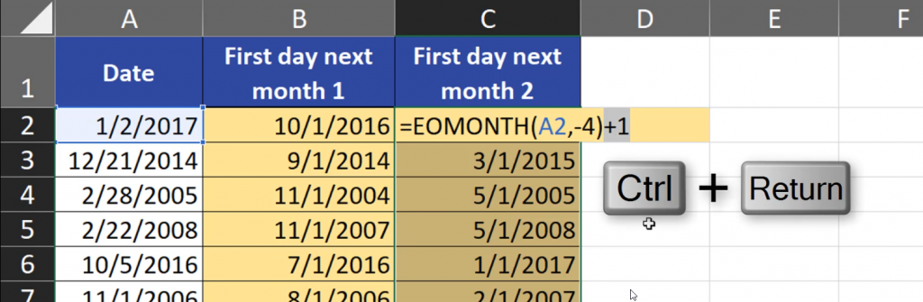
Analogically, when we want to go back in time, we need to write one month more than we really want as a negative number because we are going to the last day of the month and then we are adding 1, so in total we are going back 3 months (Fig. 14).
=EOMONTH(A2,-4)+1
Fig. 14 3 months into the past
And we have the solution (Fig. 15).
Fig. 15 Solution
The results are the same, so it’s up to you which solution you will choose.
Sometimes, we need to know what the last day of the moth is. In fact, it’s really simple to find it out because we have the end of month function — EOMONTH. This function needs a starting day and the number of moths we are moving. When we want the end of the current month, we just put 0 in the second argument of the function. Then, we must close the formula and that’s it (Fig. 1).
Last day of a month, EOMONTH function
=EOMONTH(A2,0)
Fig. 1 OEMONTH function with 0
We have the last days of current months. The EOMONTH function shows the last day even if the starting day is the last day of the month (Fig. 2).
Fig. 2 EOMONTH with current months
The EOMONTH function can move to the future. When we want to go one month into the future, we just put positive number (for example 1) instead of 0 (Fig.3).
=OEMONTH(A2,1)
Fig. 3 OEMONTH with 1
And we have the last days of the next month (Fig. 4).
Fig. 4 Last days of next months
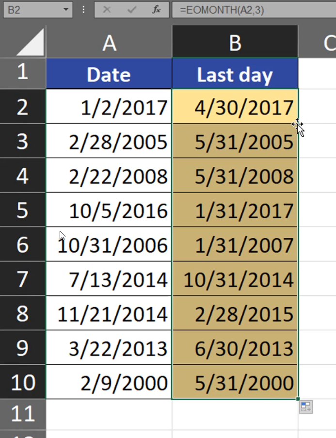
If we put a bigger number (Fig.5),
=EOMONTH(A2,3)
Fig. 5 EOMONTH with a bigger number
we will move more into the future (Fig. 6).
Fig. 6 More distant months
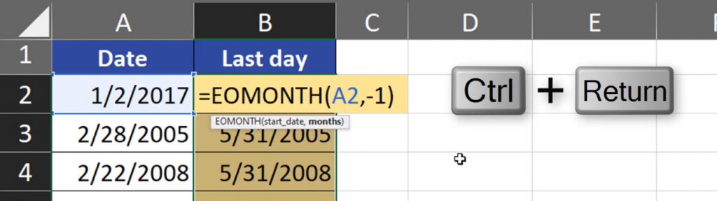
Analogically, if we want to move back in time, we just write a negative number. Let’s write ‑1 (Fig. 7).
=EOMONTH(A2, ‑1)
Fig. 7 EOMONTH with a negative number
And we are in the previous month (Fig. 8).
Fig. 8 Previous months
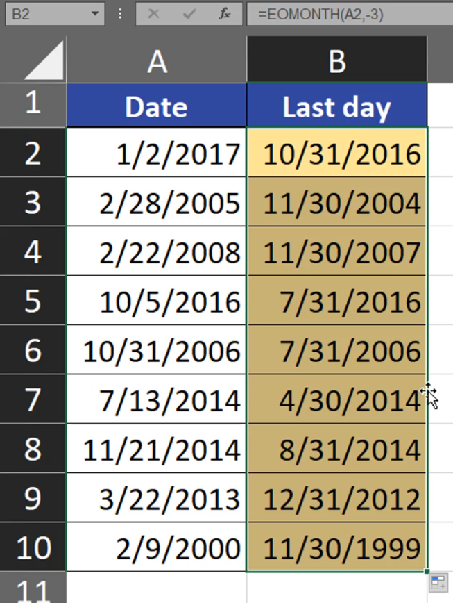
If we want to move even more into the past, we just write bigger negative numbers (Fig. 9).
=EOMONTH(A2,-3)
Fig. 9 EOMONTH with a bigger negative number
As a result, the EOMONTH function can move us even to previous or next years (Fig. 11).