Sometimes, our data is combined into one string and we want to extract only a piece of information, which will help us properly understand our data.
How to extract a date number and income from text string with a fixed width
Let’s start with extracting the date. What is important in our example, is that each string of information is of the same length, i.e. it has got a fixed width.
Fig. 1 Data of the same string lengths
We can clearly see, that the date starts with the eighth sign and has got eight signs itself (mm/dd/yy). If we want to extract a certain piece of information, we have to use the MID function. First, we have to write A2 in the argument, because our information is located in this cell. Then, we write 8 because we start with the eighth sign, and then 8 again because we want to extract eight chars. And we have our formula (Fig. 2).
=MID(A2,8,8)
Fig. 2 Formula for extracting a date
After copying it down, we have the results. It’s important though, that the MID function, just like all text functions, returns results as text. We can see it because each date is aligned to the left. It may be problematic if we want to do some date operations. We can change the text by adding 0 to our formula. In other words, we can perform any mathematical operation that won’t change the returned date (Fig. 3).
=MID(A2,8,8)+0
Fig. 3 Adding 0 to dates
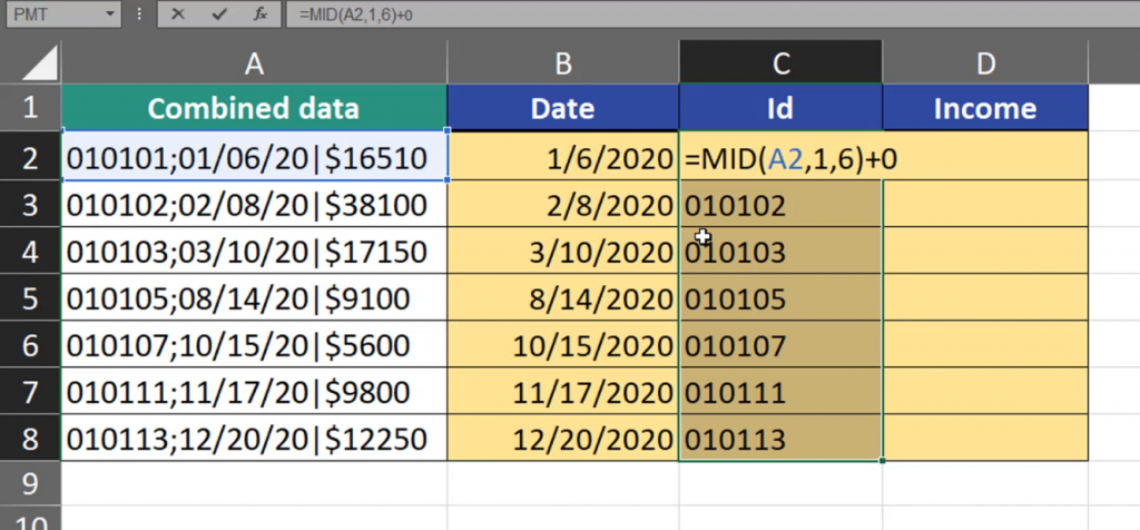
Now, we can see that the values are aligned to the right. It means that Excel treats them like numbers, i.e. like dates. We can extract Id numbers the same way. They start with the first sign and have got 6 digits in total. We can also use the MID function. First, we select cell A2, then write 1 because it starts from the first sign, then we write 6 because we extract 6 digits (Fig. 4).
=MID(A2,1,6)
Fig. 4 MID function formula for extracting Id numbers
As we can see, Excel extracted Id numbers. Since it is text, Excel left the leading zero for us. We can leave Id numbers as text if it’s important for us. If it isn’t, we can do the same as with dates, i.e. add zero (Fig. 5).
=MID(A2,1,6)+0
Fig. 5 Adding 0 to Id numbers
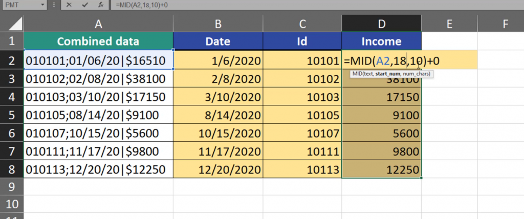
We can see that Id numbers moved to the right and the leading zero vanished. The last piece of information we want to extract is the Income. Income values don’t have a fixed width. But, since it’s the last piece of information, we can extract more signs than we need. Let’s extract also the dollar sign. The dollar sign is in the seventeenth position. We start writing the MID formula, then we add cell A2, then 17, and then we have to add the number of places we want too extract. Let’s write 10. It’s, in fact, more that we need, however it’s not less either. The MID function will extract the information to the end without any errors (Fig. 6).
=MID(A2,17,10)
Fig. 6 MID function for extracting Income
As in our previous formulas, the results are also text. By adding zero, we change the results into numbers.
MID(A2,17,10)+0
Fig. 7 Text into numbers
We can see that now the results are numbers. However, we can see that we lost the dollar sign. This is the way Excel converts numbers with dollar signs before them. Indeed, the dollar sign isn’t important in our data, so we should start from the eighteenth sign (Fig. 8).
Fig. 8 Removing the dollar sign
Now, we have only numbers. If we want to add a currency, we just go to the Home tab, drop down theGeneral bar and select the Currency option (Fig. 9).
Fig. 9 Adding a currency
When we have our results with zeros at the end, we can remove them by pressing the Decrease Decimal option (Fig. 10).
Sometimes, we want to count a certain number of weekdays between two dates. If we want to count workdays, we need to use the NETWORKDAYS function. But, if we want to count the number of, let’s say Fridays, we have to use the NETWORKDAYS.INTL function. We start with the start date, finish with the end day, and then we modify weekends. In the Excel help description, we can see that we can change working days and days off using a text string of 1s and 0s, where 1 means a day off and 0 means a working day. So, Monday, Tuesday, Wednesday, Thursday are 1, Friday is 0, Saturday and Sunday are 1 (Fig. 1).
Number of Fridays between two dates
=NETWORKDAYS.INTL(A2,B2,“1111011”)
Fig. 1 NETWORKDAYS.INTL function
Here, we have the number of Fridays between two dates. It’s important that the function also considers the start date and the end date in its calculations (Fig. 2).
Fig. 2 Number of Fridays
The NETWORKDAYS.INTL function can also work with holidays. Now, only Friday holidays are important for us, so let’s select the cell and press the F4 key to lock it (Fig. 4).
=NETWORKDAYS.INTL(A2,B2,1111011”,$F$3:$F#4)
Fig. 3 Holidays on Friday
And we have our results (Fig. 4).
Fig. 4 Results
Summing up, 0 means a working day, and 1 means a day off in the seven-number text string. If we write 0 also in the fourth place, it means that Thursday and Friday are working days (Fig. 5).
=NETWORKDAYS.INTL(A2,B2,1110011”,$F$3:$F#4)
Fig. 5 Two working days
As we can see, this small change modified our results once again (Fig. 6).
Sometimes, we want to highlight whole rows of holidays and weekends. In our case they will be the second, the third and the fourth of September, the sixth of September and so on, depending on how many holidays and weekends we have. We can highlight them with conditional formatting, but first of all, we have to create a proper formula. We are going to use the NETWORKDAYS function. We want to start with the date from the first row and finish with the same date. We also have to add holidays and lock it (Fig. 1).
=NETWORKDAYS(A2,A2,$G$2:$G$3)
If a given day is a working day, the function returns 1, and if it’s a day off, it returns 0 (Fig. 2).
Fig. 2 Working days and days off
Now, we want to highlight the rows, where we have 0. We can do it by creating a proper logical test. We have to check whether a value returned by the NETWORKSDAYS function is equal to 0 (Fig. 3).
=NETWORKDAYS(A2,A2,$G$2:$G$3)=0
Fig. 3 A simple logical test
Now, we want to ask ourselves how we want our reference to behave. Since we want to copy the formula down, we want to change rows, as there are different dates in each row. We also want to highlight a whole row, so we always want to look at the first cell in the row because it’s a date. Having this in mind, we have to lock the column by inserting a single dollar sign before the name of the column, but not before the row number. We must do this both in the start date and the end date argument (Fig. 4).
Fig. 4 Locked cell
After copying it down and to the right, we have proper results. We have TRUE for weekends and holidays, and FALSE for working days (Fig. 5).
Fig. 5 Proper results of TRUE and FALSE
Now, we can copy our formula in the edit mode and select the range in which we want to have conditional formatting. We click on the Shift + →, two times to the right, and Ctrl + Shift + ↓ to select the data to the end. While cell A2 is still active, we can go to Home tab, then Conditional Formatting, then the New Rule option (Fig. 6).
Fig. 6 New Rule option
In the New Rule Formatting window, we have to select the Use a Formula to determine which cells to format bar, then paste the formula into the Edit the Rule Description bar, and click on the Format tab (Fig. 7).
Fig. 7 New Formatting Rule window
In the Format Cells window, we select the Fill tab, then choose a nice color, then press the OK button in the window, then the OK button in the second window (Fig. 8).
Fig. 8 Format cells window
And there we have it. We can see that each row with a day off is highlighted in green (Fig. 9)
Fig. 9 Highlighted rows
Even if we modify the holidays, which are our criteria, our highlighted rows also change (Fig. 10).
If you want to find a date after a certain number of workdays, you can use the WORKDAY function. You just need the start date and the number of working days (Fig. 1).
Date after X work daysFig. 1 WORKDAY function
We can see that Excel shows the date after the corresponding number of working days. You have to remember that the WORKDAY function doesn’t consider the start date in its calculations. It means that if you have only one workday, you will go to the next working day (Fig. 2).
Fig. 2 Next working day
In the WORKDAY function, you can even add holidays by just selecting a range with proper dates. Remember to lock it (F4) (Fig. 3).
Fig. 3 Adding holidays
We can see that our dates are a bit changed (Fig. 4).
Fig. 4 Dates changed
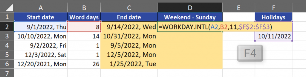
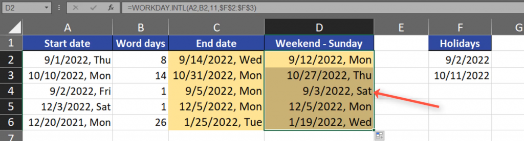
The WORKDAY function considers the weekend as Saturday and Sunday, which is correct in most of the countries, however we can modify it. When we want only Sunday to be our weekend, we have to choose the WEEKDAYS.INTL function. The function consists of the start date and the number of working days. The third argument is the weekend, where we can change the weekend days. Let’s choose Sunday (Fig. 5).
Fig. 5 Sunday as the weekend
Then, we are choosing holidays by selecting a proper range and locking it (F4 key). Our formula is ready (Fig. 6).
=WORKDAY.INTL(A2,B2,11,$F$2:$F$3)
Fig. 6 Our formula
We can see that our results differ from the the previous ones because now Saturday is our working day (Fig. 7).
When we want to count the number of working days between two dates we can use the NETWORKDAYS function. The function is very simple, as it needs only the start and end dates. And that’s it (Fig. 1).
Number Of Working Days Between Two Dates
=NETWORKDAYS(A2,B2)
Fig. 1 NETWORKDAYS function
And we have the numbers of working days between two dates. It’s important that the NETWORKDAYS function considers also the start and end days. If the start and end days are the same, the number will tell us whether the day is a working day or not (Fig. 2).
Fig. 2 Working days
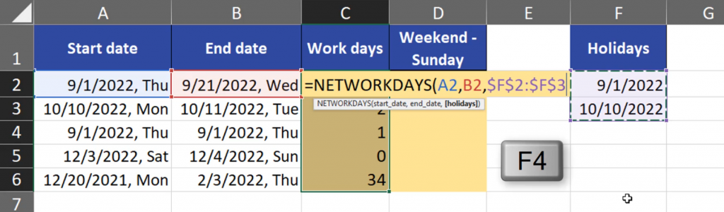
We can also add holidays to this function in the third argument. We just have to select a range with proper dates and press the F4 key to lock it (Fig. 3).
=NETWORKDAYS(A2,B2,$F$2:$F$3)
Fig. 3 Holidays
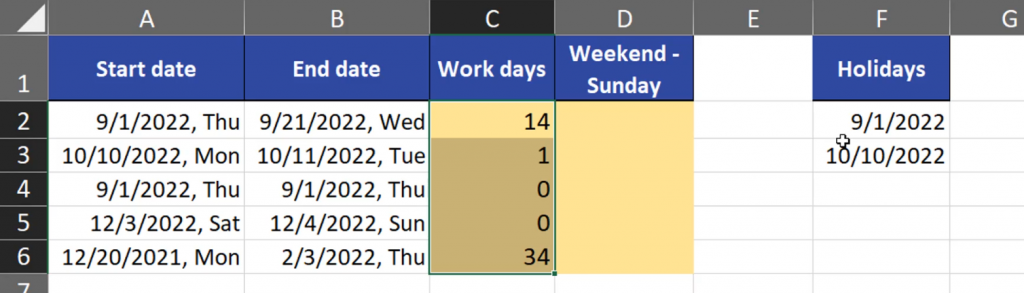
Now, we can see that the number of days changed due to those holidays (Fig. 4).
Fig. 4 Changed numbers
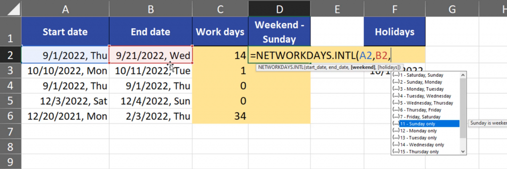
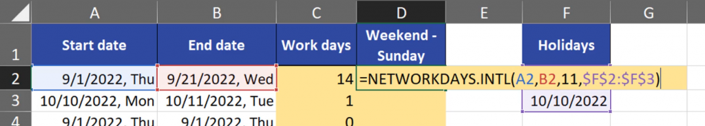
In the NETWORKDAYS function, the weekend is considered as Saturday and Sunday. However, we can modify it by using the NETWORKDAYS.INTL function. The syntax of those two functions is almost the same. Apart from the start and end day, we can choose what our weekend days will be. Let’s choose Sunday only (Fig. 5).
Fig. 5 NETWORKDAYS.INTL function
Then, we can add holidays if we want. Let’s select the proper holiday range and press the F4 key to lock it (Fig. 6).
=NETWORKDAYS.INTL(A2,B2,11,$F$2:$F$3)
Fig. 6 Function with holidays
And we have our results. We can see that the number of working days between the dates grew because Saturday is a working day (Fig. 7).