Named ranges and statistics

Some­times, we need to make many sta­tis­ti­cal oper­a­tions and use many sta­tis­ti­cal func­tions in Excel. How can we do it?

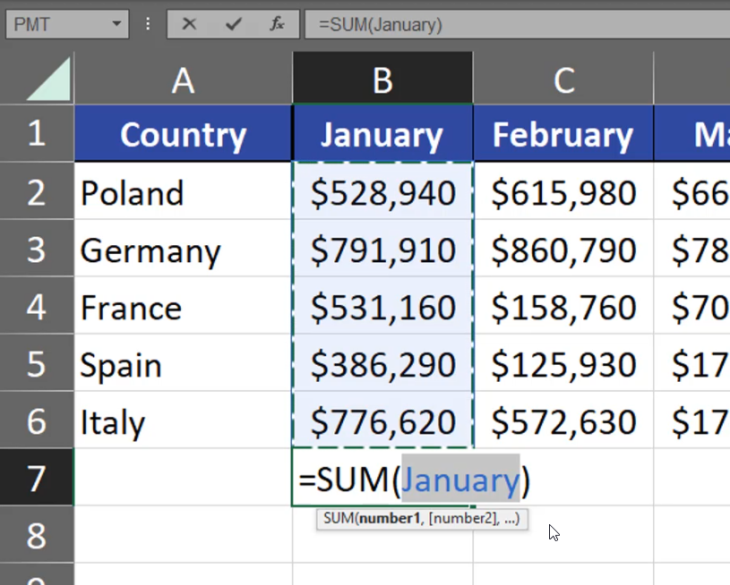
A fast and quick solu­tion is using name ranges. For exam­ple, we have the SUM func­tion that sums up all val­ues from Jan­u­ary (Fig. 1)

How can we name ranges and use them for our advan­tage? Let’s start with a sim­ple exam­ple of the SUM func­tion. For the SUM func­tion, we have key­board short­cut which is Alt + =. This way Excel will put the sum for Jan­u­ary, which is a range form B2:B6 (Fig. 2)

=SUM(B2:B6)

In the exam­ple above we had num­bers. How­ev­er, let’s go to anoth­er sheet where we have no num­bers. When we want to sum the num­bers from the pre­vi­ous sheet, it’s going to be a very tedious job, as we have to move between those two sheets and write prop­er val­ues. What’s more, the ref­er­ence we have while using val­ues form anoth­er sheet isn’t the eas­i­est to under­stand. What we can do is nam­ing the ranges. We just have to select a range in a col­umn and write a prop­er name in the Name Box (Fig. 3).

Now, when we are using the Alt + = short­cut under our val­ues, Excel will auto­mat­i­cal­ly refer to the Jan­u­ary range, which is B2:B6 (Fig. 4)

=SUM(Jan­u­ary)

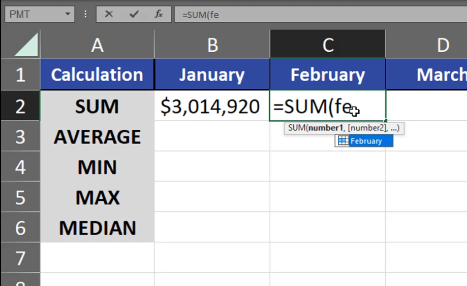
As we know, Excel remem­bers names. It means that we can use the name in cal­cu­la­tion on a dif­fer­ent sheet. When I start writ­ing “ja” in anoth­er sheet, Excel will sug­gest the range name (Fig. 5). I can just accept it and sum the val­ues from January. 

As we can see, nam­ing ranges makes our work faster. We can also name a big­ger group of columns at one time. Just select the group you want. What’s impor­tant, when you’re select­ing your data, you have to select the top rows, and then the num­bers beneath them. Then, go to the For­mu­las tab, click on the Cre­ate from Selec­tion com­mand and select the Top Row check­box in the win­dow that appeared (Fig. 6)

Now, after we named our ranges, we can see that the Feb­ru­ary range is named Feb­ru­ary, the March range is named March and so on. When we move to anoth­er sheet, we can use those names (Fig. 7)

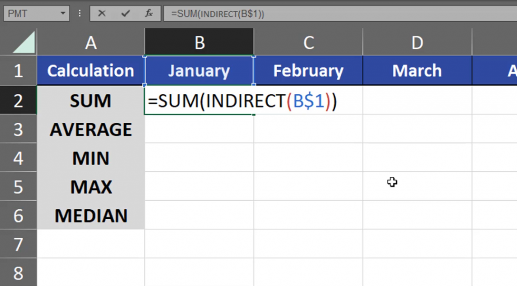
How­ev­er, we can go one step fur­ther using the ref­er­ence to names. I have Jan­u­ary in cell B1. But, when I refer to cell B1, Excel won’t sim­ply con­vert the text from cell B1 to a range because it just text. It means that our func­tion won’t add any­thing. First of all, we have to lock the rows (B$1), then add the INDIRECT func­tion to our cal­cu­la­tion. Now, the INDIRECT func­tion changes the text into a ref­er­ence to the prop­er range (Fig. 8)

=SUM(INDIRECT(B$1))

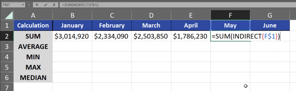
Now, when I drag the for­mu­la to the right, I will have sums from each indi­vid­ual month (Fig. 9)

=SUM(INDIRECT(F$1))

When I copy the for­mu­la one cell low­er, I’m just chang­ing SUM into AVERAGE (Fig. 11)

=AVERAGE(INDIRECT(B$1))

After I drag it to the right, I have prop­er results. I do the same with the remain­ing rows (Fig. 12)

=MIN(INDIRECT(B$1))

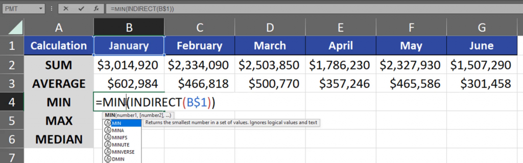
This way, we can quick­ly add more sta­tis­ti­cal oper­a­tions for many months using prop­er name ranges and the INDIRECT function. 

https://www.youtube.com/watch?v=E9APUsy4y‑E