How to calculate a sum or an average of top 3 maximal values?
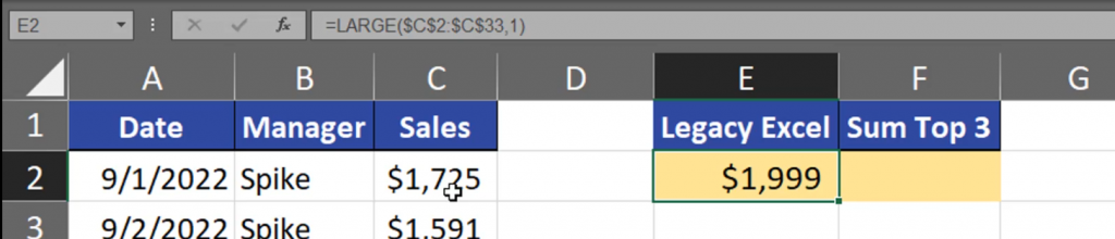
In Legacy Excel, we can use the LARGE function, in which we need to select the range for our calculation. In the k argument let’s write 1 (Fig. 1).
=LARGE($C$2:$C$33,1)

After entering the function, we have the largest value (Fig. 2).
Now, we can copy the function and add the second and the third largest value (Fig. 3).
=LARGE($C$2:$C$33,1)+LARGE($C$2:$C$33,2)+LARGE($C$2:$C$33,3)

This way we have the sum of 3 largest values (Fig. 4).

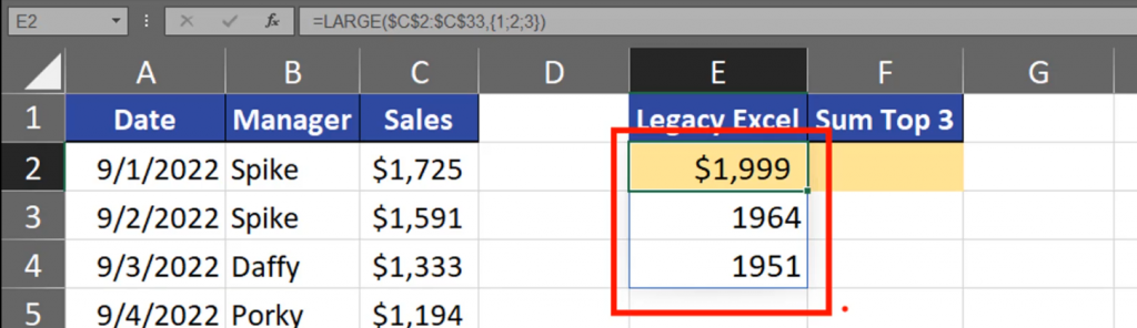
This solution, however, is the least dynamic of all solutions we have. We can make this formula shorter by hardcoding our values. We have to write 1, 2 and 3 as an array (Fig. 5).
=LARGE($C$2:$C$33,{1;2;3})

This way Excel will return three largest values. I’m using Dynamic Excel, so the results are spilled (Fig. 6).
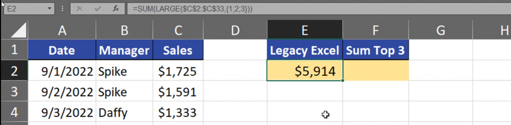
Now, that our values have been hard-coded, we can sum them by using the SUM function. We can also use this function to sum up averages (Fig. 7).
=SUM(LARGE($C$2:$C$33,{1;2;3}))

Our results (Fig. 8).
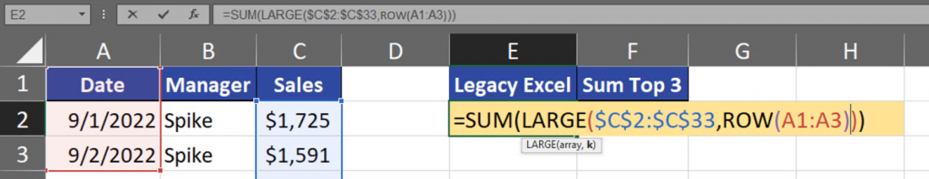
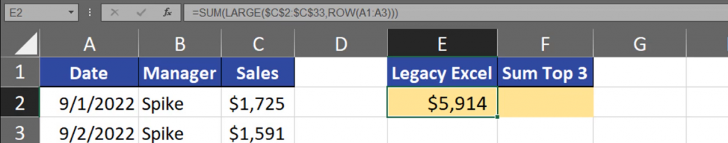
This solution, however, is hard to modify, so we can make it a bit more dynamic. We can use the ROW function and select the first three rows from the sheet. This way our solution is more dynamic (Fig. 9).
=SUM(LARGE,($C$2:$C$33,ROW(A1:A3)))
Results (Fig. 10).
But, in Legacy Excel, we should use the SUMPRODUCT function instead of the SUM function or use the Ctrl + Shift + Enter shortcut to put the formula into the cell (Fig. 11).
=SUMPRODUCT(LARGE,($C$2:$C$33,ROW(A1:A3)))

And we have the result. In the second column, in Dynamic Array Excel, we still need the SUM and LARGE functions, then the array which is the range we will look at. Then, we can use the SEQUENCE function to create a sequence of proper numbers, let’s take 3 (Fig. 12).
=SUM(LARGE($C$2:$C$33,SEQUENCE(3)))
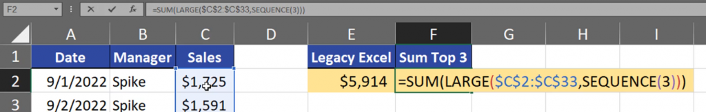
We have proper results (Fig. 13).

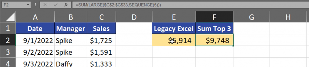
This solution is much more dynamic. Let’s change the number into 5 (Fig. 14).
=SUM(LARGE($C$2:$C$33,SEQUENCE(5)))

Here is the result (Fig. 15).
In Legacy Excel, we can also change one number. Let’s change the number of rows in the range from 3 to 5 (Fig. 16).
=SUMPRODUCT(LARGE($C$2:$C$33,ROW(A1:A5)))

And we have the same result (Fig. 17).

We have to remember which version of Excel we have and which solution we can use.