Sometimes, you need to create a running total in pivot tables. How to do it properly?
Let’s start with creating a pivot table. Select one cell from our data and go to the Insert tab and select the Pivot Table command. A Pivot table from table or range window will appear, where we have our range. We need to select the Existing worksheet radio button and write the location, which, in our case, will be cell F1. Let’s click the OK button (Fig. 1).

And there we have it. In our pivot table we need to drag the Date to the Rows labels.

Now, depending on the Excel version, we have an option of Group by dates. I’m going to group our date by months and years (Fig. 3).

We have our table. Now, I want to add Income so let’s press the Income checkbox (Fig. 4).

Now, I want to have the income and the running total for the income, so let’s drag the Income two times to the Values area. We can see that we have Sum of Income and Sum of Income 2, where we actually want to have our running total (Fig. 5).

Let’s right click any value from Income 2, then select the Show Values as and then the Running Total In option (Fig. 6).

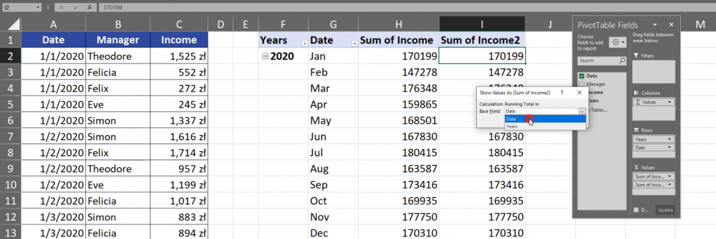
Now, we have to decide whether we want to base our running total on Date or Years Field. Let’s take Date (Fig. 7).
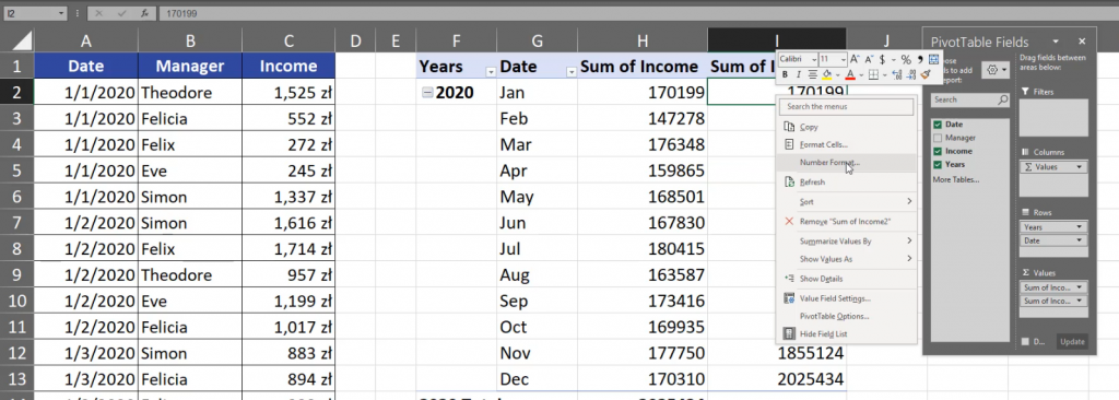
Now, we can see that in the Income 2 column we have bigger numbers. Let’s format them by pressing any cell in the column and choosing the Number Format option (Fig. 8).
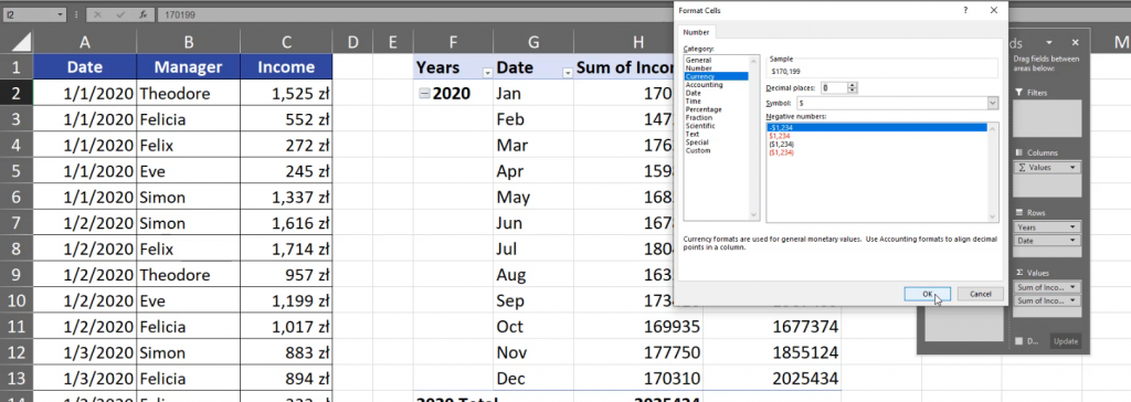
In the Format Cell window, let’s choose the Currency category, in Decimal places let’s write 0 and press the OK button. Let’s do the same in the Sum of Income column (Fig. 9).
Now, we can see that we are working with money. In each month we have bigger and bigger numbers which means that we have the running total in this column. We can change the name of Sum of Income 2 into Running Total. Since we are using the Date Field as our reference point, we have the running total in 2020. In 2021 Excel counts from the start, which means that we have the running total only for 2021. The same is with 2022. If we change the Date field into the Years field in the Show Values as (Running Total) window, we will have the same value in the first year and in the Sum of Income column (Fig. 10).

However, in the next year, we have the the sum from January 2021 and January 2020. In February, we have the sum from February 2021 and 2020. In 2022, we have sums from three Februaries (Fig. 11).

Let’s drag Manager into the columns header (Fig. 12).
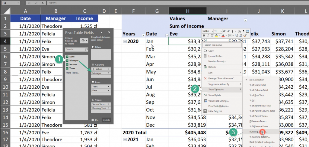
By doing so, we can show value from the Manager’s perspective, which means a horizontal view.

However, this type of data isn’t a proper one to show it this way, so let’s get back by pressing Ctrl + Z two times and see that we can also create a percent running total by going to the % Running Total In option and choose the Date Field (Fig. 14).

Now, we can see the values as percentage (Fig. 15).
