Extract First Last and Middle Name with Formulas 

Today, we are going to talk about extract­ing first names, mid­dle names and last names from full names. We define the first name as the first word from the left, the last name as the first word from the right, and the mid­dle name, as every­thing between those two. Mid­dle names are a bit com­pli­cat­ed, as they can may con­sist of one word, a space, an abbre­vi­a­tion, or two or more words (Fig. 1)

Let’s start with extract­ing the first name. We just have to use the LEFT func­tion, which extracts signs from the left. We have to insert the FIND func­tion there, so that it finds the first space, and write the space in dou­ble quotes (Fig. 2)

=LEFT(A2,FIND(“ “,A2))

Now, we have the first name (Fig. 3).

But, we have to remem­ber that the FIND func­tion will return the posi­tion of the sign we’re look­ing for, which means that it finds the 7th posi­tion, which is a space (Fig. 4). 

The first name , how­ev­er, con­sists of only 6 let­ters, which is what we want. It means that we want to extract less let­ters. So, we have write the for­mu­la once again, but this time we sub­tract one sign (Fig. 5)

=LEFT(A2,FIND(“ “,A2)-1)

Now, we have only the first name with­out unnec­es­sary signs. After drag­ging it down, the whole col­umn is full (Fig. 6)

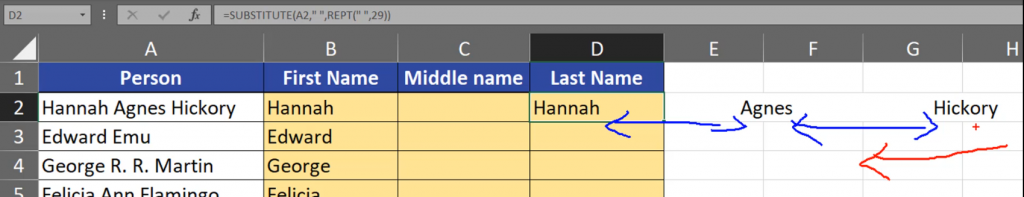
Let’s go to last names. This case is a bit more com­pli­cat­ed. We don’t know whether we’re look­ing for the first, the sec­ond, the third or even a more dis­tant space (Fig. 7) 

There’s a trick to solve it. We have to repeat spaces. With­in our text, we have to sub­sti­tute a sin­gle space into many spaces, let’s say 29. We use the REPT func­tion (Fig. 8)

=SUBSTITUTE(A2,” “,REPT(“ “,29))

After accept­ing our func­tion, we have our changed names with many spaces between them (Fig. 9)

Now, we can start extract­ing names from the right side. We’re extract­ing not only all signs from our name, but also the remain­ing 29 signs (Fig. 10).

=RIGHT(SUBSTITUTE(A2,” “,REPT(“ “,29)),29)

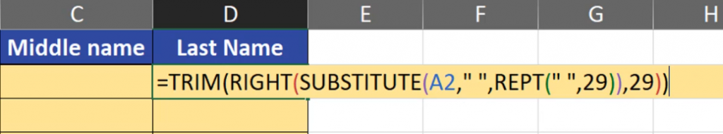
Now, we have the last name and many, many spaces before it (Fig. 11)

We have to delete them using the TRIM func­tion. The TRIM func­tion removes all spaces from a text string except for a sin­gle space between words. So, each space at the begin­ning and at the end of the string will be removed (Fig. 12)

=TRIM(RIGHT(SUBSTITUTE(A2,” “,REPT(“ “,29)),29))

After accept­ing it and copy­ing it down, we have our last names (Fig. 13). 

Now, we have to find the thing between the first and the last name. We will use the SUBSTITUTE func­tion. In the place of the first name, we will place noth­ing, i.e. an emp­ty text string (Fig. 14). 

=SUBSTITUTE(A2,B2,“”)

Now, we have a short­er ver­sion of our name (Fig. 15).

Let’s remove the last name now. We want to sub­sti­tute the last name with an emp­ty text string (Fig. 16)

=SUBSTITUTE(SUBSTITUTE(A2,B2,“”),D2,“”)

After enter­ing and copy­ing down, we have every­thing between the first name and the last name (Fig. 17). As you can see, we have also extract­ed spaces which we don’t need. So, let’s use the TRIM func­tion to delete unnec­es­sary spaces.

=TRIM(SUBSTITUTE(SUBSTITUTE(A2,B2,“”),D2,“”))

Because we are edit­ing whole col­umn we can press Ctrl + Enter.

That’s how we extract first names, last names and every­thing in between with appro­pri­ate formulas. 

https://www.youtube.com/watch?v=v46vQGjwx0w