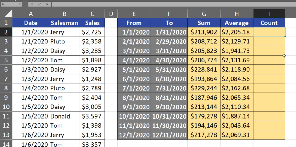
Today, we are counting sums, averages and number of transactions with more than one condition. In our example, we have transaction sales table and we want to count the values for given months. However, the months are written as the first day of the month and the last day of the month. It means that we have to add two conditions in order to count it. Let’s start with sums. We can use the SUMIFS function. The first argument of this function is a range on which we will be summing. In our case it’s the sales column so we have to select cell C2 and press the Ctrl + Shift + ↓ combination, then the F4 key to lock it (Fig. 1).
=SUMIFS($C$2:$C$1193

We write a comma, and then we are going to the criteria range 1. This will be the range where we will be checking the first criterion, which is the third argument of the SUMIFS function. In our case, we are checking dates, so let’s press cell A2, Ctrl + Shift + ↓, then the F4 key. We are adding a comma again, and now we have to write the first condition, which is the first criterion. The order of our conditions is not important because, in the end, all conditions have to be met to count the thing we want. Let’s start with the From date. We want values that are bigger or equal to this date, which means that we have to write the symbols of larger than and equal in double quotes, then an ampersand because we are combining this text with the value from cell E2 (Fig. 2).
=SUMIFS($C$2:$C$1193,$A$2:$A$1193,”>=”&E2

After pressing the F9 key, we can see that Excel changed the date into a number. This makes Excel check our condition properly (Fig. 3).
=SUMIFS($C$2:$C$1193,$A$2:$A$1193,“>=43831”

However, let’s move back to previous text by pressing Ctrl + Z. Now, we have the first condition. We can see that the second condition is necessary with second critirion because the next two arguments are in square brackets (Fig. 4).
=SUMIFS($C$2:$C$1193,$A$2:$A$1193,”>=”&E2

Criteria range 2 in our case is the same as criteria range 1, so we can just copy it (Ctrl +C, Ctrl +V), but we really need to put it because each criteria range is working just with the argument of its criteria. It means that criteria range 1 is working with criteria 1, and criteria range 2 is working with criteria 2. In our case, the criteria 2 are numbers smaller than or equal to the last day of the month in cell F2.
Now, we have the whole formula (Fig. 5).
=SUMIFS($C$2:$C$1193,$A$2:$A$1193,”>=”&E2,$A$2:$A$1193,”<=”&F2)

When we want to sum the values from the sum range, the first and the second condition have to be met. Let’s put the formula and copy it down. We can see that at the end everything is working properly because we have written the formula properly (Fig. 6).

We still have some more values to count. Let’s take the averages. Since I’m a lazy person, I will copy the whole formula in edit mode, then go to the Average column, paste it and change only the name of SUMIFS into AVERAGEIFS. After entering it, we can see that only the sum range changed its name into average range. The remaining argument names stayed the same. It’s because the SUMIFS and the AVERAGEIFS formulas have the same syntax, but they count sums and averages correspondingly (Fig. 7).

Let’s put the formula into our cell and copy it down. We have the results (Fig 8).
Let’s now count the number of transactions. We will use the COUNTIFS function. This function doesn’t have any range on which we could count sums, averages and so on. It only needs criteria ranges and criteria. Our first criteria was the one with dates. So, let’s write A2, then press Ctrl + Shift + ↓, then the F4 key to lock it and a comma. I want to show you that the order of conditions is not important. Let’s take values smaller that or equal to the date in cell F2, comma, then the same criteria range, then the second criteria will be greater than or equal to the value from cell E2. Those are all the arguments we need for a COUNTIFS function (Fig. 9).
=COUNTIFS($A$2:$A$1193,”<=”&F2,$A$2:$A$1193,”>=”&E2)

After copying the formula down, we have the results. We can check if our average is correct just by looking at it because it is just the sum divided by the number of transactions (Fig. 10).

We can see that the numbers are exactly the same as in the Average column (Fig. 11).
